Maintenance Policies Corrective maintenance It is usually referred

Maintenance Policies • Corrective maintenance: It is usually referred to as repair. Its purpose is to bring the component back to functioning state as soon as possible. In some cases, it involves replacement of one or more components. • Preventive maintenance: Its purpose is to reduce the probability of component failure. It may involve lubrication, small adjustment, or replacing components or parts of components that are beginning to wear out. Periodic testing and maintenance based on condition monitoring are also regarded as preventive maintenance.

Maintainability The ability of an item, under stated conditions of use, to be retained in, or restored to, a state in which it can perform its required functions, when maintenance is performed under stated conditions and using prescribed procedures and resources (BS 4778).

Availability The ability of an item (under combined aspects of its reliability, maintainability, and maintenance support) to perform its required function at a stated instant of time or over a stated period of time (BS 4778). When considering a production system, the average availability of the production is sometimes called the production regularity.

Corrective Maintenance Replacement/repair after failure

Transition of Component States Normal state continues Component fails N F Component is repaired Failed state continues

The Failure-to-Repair Process

Repair Probability - G(t) • The probability that repair is completed before time t, given that the component failed at time zero. • If the component is non-repairable

Repair Density - g(t)

Repair Rate - m(t) • The probability that the component is repaired per unit time at time t, given that the component failed at time zero and has been failed to time t. • If the component is non-repairable

Mean Time to Repair - MTTR

The Whole Process

Availability - A(t) • The probability that the component is normal at time t, i. e. , A(t)=Pr{X(t)=1}. • For non-repairable components • For repairable components

Unavailability - Q(t) • The probability that the component fails at time t, i. e. , • For non-repairable components • For repairable components

Unconditional Failure Density, w(t) The probability that a component fails per unit time at time t, given that it jumped into the normal state at time zero. Note, for non-repairable components.

Unconditional Repair Density, v(t) The probability that the component is repaired per unit time at time t, give that it jumped into the normal state at time zero.

Conditional Failure Intensity λ(t) The probability that the component fails per unit time, given that it is in the normal state at time zero and normal at time t. In general , λ(t)≠r(t). For non-repairable components, λ(t) = r(t). However, if the failure rate is constant (λ) , then λ(t) = r(t) = λ for both repairable and nonrepairable components.

Conditional Repair Intensity, µ(t) The probability that a component is repaired per unit time at time t, given that it is jumped into the normal state at time zero and is failed at time t, For non-repairable component, µ(t)=m(t)=0. For a constant repair rate m, µ(t)=m.

The Average Availability The average availability in a time interval is defined as This definition can be interpreted as the average proportion of interval where the component is able to function.

The Limiting Availability It can be shown that In the reliability literature, the symbol A is often used as notation both for the limiting availability and the average availability.

Expected Number of Failures (ENF)

ENF over an interval, W(t 1, t 2 ) Expected number of failures during (t 1, t 2) given that the component jumped into the normal state at time zero. For non-repairable components

ENR over an interval, Expected number of repairs during , given that the component jumped into the normal state at time zero. For non-repairable components

Mean Time Between Repairs, MTBR Expected length of time between two consecutive repairs. MTBR = MTTF + MTTR Mean Time Between Fails, MTBF Expected length of time between two consecutive failures. MTBF = MTBR

Let where

r(t)= Const. ● Failure Rate r(t) General r(t) RELATIONS AMONG PROBABILISTIC PARAMETERS FOR REPAIR-TO-FAILURE PROCESS (THE FIRST FAILURE)

m(t)=u General m(t) Const. Repair Rate m(t) RELATIONS AMONG PROBABILISTIC PARAMETERS FOR FAILURE-TO-REPAIR PROCESS ●

RELATIONS AMONG PROBABILISTIC PARAMETERS FOR THE WHOLE PROCESS Repairable Non-repairable ◎ Fundamental Relations ※ ※ ※ ( Next )

Remark Stationary Values

CALCULATION OF w(t) and v(t) (given f (t) and g (t)) Two types of components fail during [t, t+dt] : F Type I N F N Type II time u u+du Probability of Type I : ( v (u) du ) ( f (t-u) dt ) Probability of Type II : f (t) dt OR t t+dt

One type of components which is repaired during [t, t+dt] F N u u+du OR t t+dt time

[ EXAMPLE ]

0 18 1 0 0 1 18 1 0 3 0. 1667 2 15 0. 8333 0. 1667 10 0. 5556 0. 6667 3 5 0. 2778 0. 7222 1 0. 0556 0. 2001 4 4 0. 2222 0. 7778 2 0. 1111 0. 5000 5 2 0. 1111 0. 8889 1 0. 0556 0. 5005 6 1 0. 0556 0. 9444 0 0 0 7 1 0. 0556 0. 9444 1 0. 0556 1. 0000 8 0 0 1 0 0 - 9 0 0 1 0 0 -

assumption TTF data Exponential Weibull Normal Log-normal Histogram polynomial approximation parameter identification f (t) r (t) F (t) R (t) MTTF

assumption TTR data Exponential Weibull Normal Log-normal Histogram Polynomial approximation parameter identification g (t) m (t) G (t) MTTR

f (t), g (t) or w(0) = f(0), v(0) = 0 w (t), v (t) Q (t) A (t) = 1 - Q (t) A (t)

Constant-Rate Models • Repair-to-Failure

NON-REPAIRABLE 1 Good Failed P (t) = probability that the component is good at time t = R(t) good at t and remained good failed at t and was repaired Initial Condition :

Constant-Rate Models • Failure-to-Repair

Constant-Rate Models • Dynamic Behavior of Whole Process (1) • also

REPAIRABLE 1 -λΔt 1 -μΔt Good λΔt good and remained good Failed failed and repaired

Initial Condition: P(0)=1

Constant-Rate Models • Dynamic Behavior of Whole Process (2)

Constant-Rate Models • Stationary Values of the Whole Process

Proof (1) • From • Laplace Transform

Proof (2) • Rearrangement and Inversion

System Availability

Approximate Average (Limiting) System Unavailability

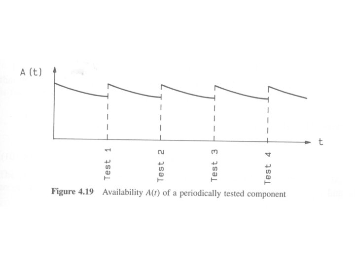
Preventive Maintenance Periodic Testing and/or Replacement

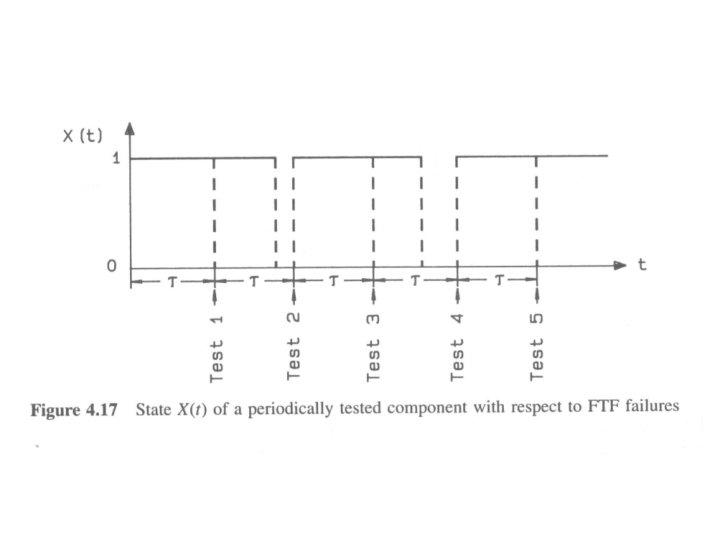
The Hidden Failures • The protective devices, i. e. alarms, SVs, interlocks and trips, are passive components. • There are two failure modes: “fail to function” (FTF) and “false alarm” (FA). The most important failure mode is (FTF) and is always a hidden failure. • The maintenance policy of periodic testing, and repair or replacement is often needed to improve the reliability of components with hidden failures. After a test (repair), the component is considered to be “as good as new. ”

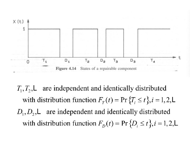
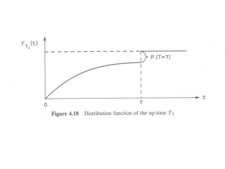
The Component Up-Time • Let T be the time to FTF failure of a component, with distribution function and probability density • Consider the first test interval (0, ]. Let be the part of this time interval where the component is able to function and be the part where the component fails.

The Distribution of Up-Time It should be noted that these function are periodical. In other words, they are the same in the intervals

The Average Availability • Consider the first test Interval (0, ], it can be shown that • Since all test intervals have the same stochastic characteristics,

The Mean Fractional Dead Time (MFDT) The average unavailability is often called the mean fractional dead time, i. e.

Special Case – Constant Failure Rate • Mean Up-Time

Special Case – Constant Failure Rate • Average availability • Mean fractional dead time

Special Case – Constant Failure Rate • Expansion • Approximation

Example

System Unavailability • Consider a system of n independent components with constant failure rates, • Failures in a test interval are neither detected nor repaired. Hence the component may be regarded as nonrepairable within the test interval.

System Unavailability • The cut set unavailability • The system unavailability where denotes the order of the minimal cut set and j = 1, 2, …, k.

The System MFDT

The k-out-of-n System Assume that there are n identical and independent system with constant failure rate. The system has C(n, n-k+1) cut sets of order (n-k+1).

MFDT of k-out-of-n Systems kn 1 2 3 1 2 --- 3 4 --- --- --- 4

Mean Time to Failure • Let denote the time from the component is put into operation until its first failure where, Z is the number of test intervals until the component fails for the first time; is the down time in interval (0, τ).

The mean number of test intervals until the component fails – E[Z]

The Mean Down Time =F(τ) 0

Mean Time to Failure • Special Case: constant failure rate

The Critical Situation • • • A critical situation occurs if a hazardous event occurs while the protective system is in a failed state. The hazard rate is constant β. A critical situation occurs in (0, τ] if 1. The protective system fails in (t, t+dt] where t<τ and, simultaneously 2. At least one hazardous event occurs in (t, τ].

The Probability of Critical Event • The probability of at least one critical event in the interval (0, τ] is • Since and MFDT