Magnetosphere and Ionosphere Models Masha Kuznetsova CCMCNASA GSFC

Magnetosphere and Ionosphere Models Masha Kuznetsova CCMC/NASA GSFC http: //ccmc. gsfc. nasa. gov R 2 O Workshop October 15 -18, 2007

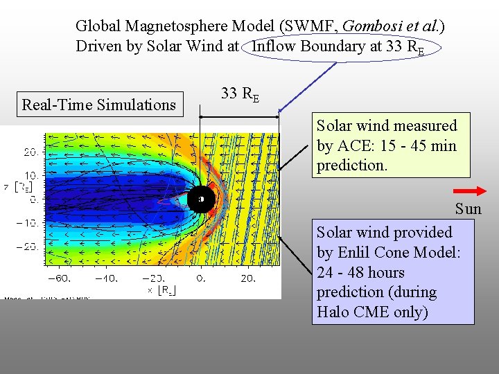
Global Magnetosphere Model (SWMF, Gombosi et al. ) Driven by Solar Wind at Inflow Boundary at 33 RE Real-Time Simulations 33 RE Solar wind measured by ACE: 15 - 45 min prediction. Sun Solar wind provided by Enlil Cone Model: 24 - 48 hours prediction (during Halo CME only)

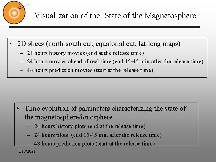
Visualization of the State of the Magnetosphere • 2 D slices (north-south cut, equatorial cut, lat-long maps) – 24 hours history movies (end at the release time) – 24 hours movies ahead of real time (end 15 -45 min after the release time) – 48 hours prediction movies (start at the release time) • Time evolution of parameters characterizing the state of the magnetosphere/ionosphere – 24 hours history plots (end at the release time) – 24 hours plots (end 15 -45 min after the release time) – 48 hours prediction plots (start at the release time) 3/10/2021

Overview of the Global State of the Magnetosphere: North-South Cut Magnetopshere hit by CME Density (color, log scale), Velocity (vectors), Magnetic field (lines) Quiet magnetopshere Substorm onset reconnection onset 3/10/2021 Near-earth reconnection causes energetic particle injection at geosynch. orbit, drive geomagnetically induced currents.

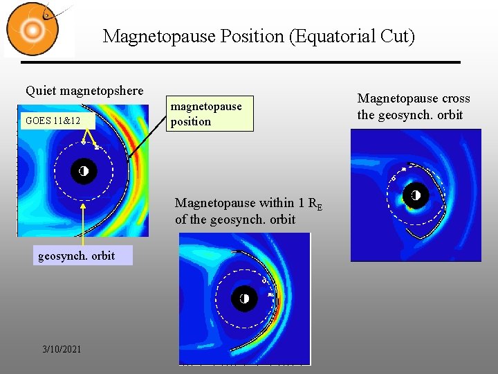
Magnetopause Position (Equatorial Cut) Quiet magnetopshere GOES 11&12 magnetopause position Magnetopause within 1 RE of the geosynch. orbit 3/10/2021 Magnetopause cross the geosynch. orbit

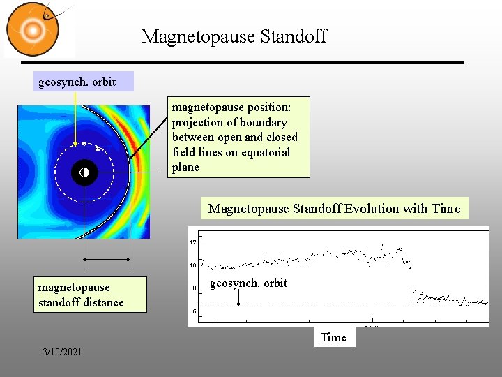
Magnetopause Standoff geosynch. orbit magnetopause position: projection of boundary between open and closed field lines on equatorial plane Magnetopause Standoff Evolution with Time magnetopause standoff distance geosynch. orbit Time 3/10/2021

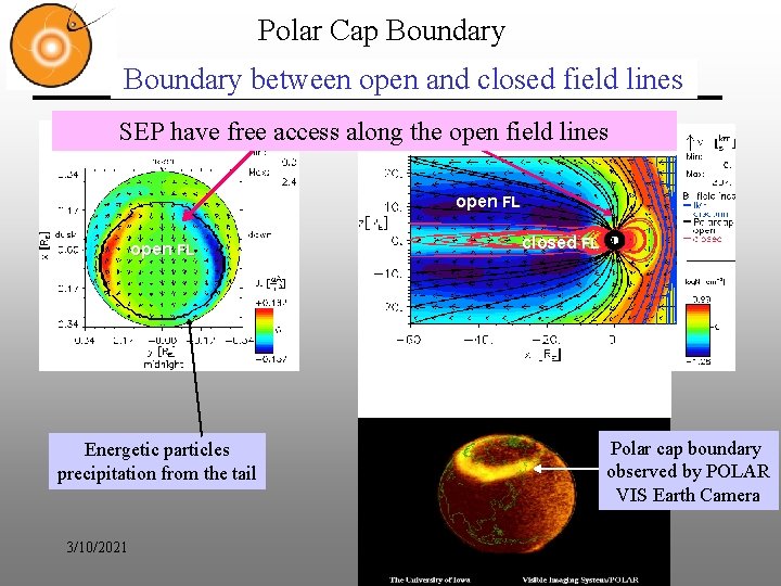
Polar Cap Boundary between open and closed field lines SEP have free access along the open field lines open FL Energetic particles precipitation from the tail 3/10/2021 closed FL Polar cap boundary observed by POLAR VIS Earth Camera

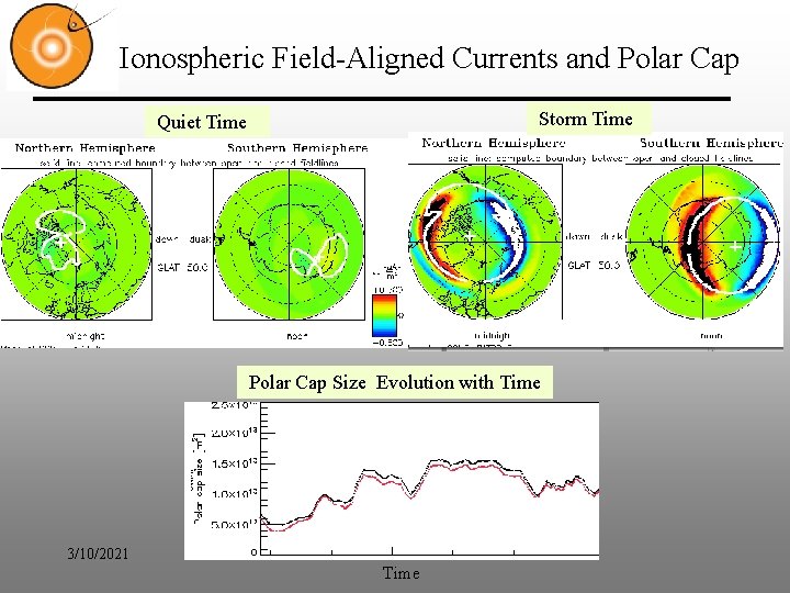
Ionospheric Field-Aligned Currents and Polar Cap Storm Time Quiet Time Polar Cap Size Evolution with Time 3/10/2021 Time

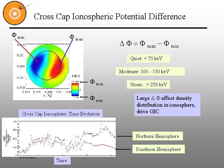
Cross Cap Ionospheric Potential Difference F min F max D F = F max - F min Quiet: < 75 ke. V Moderate: 100 - 150 ke. V F max F min Cross Cap Ionospheric Time Evolution Storm: > 250 ke. V Large D F affect density distribution in ionosphere, drive GIC Northern Hemisphere Sourthern Hemisphere 3/10/2021 Time

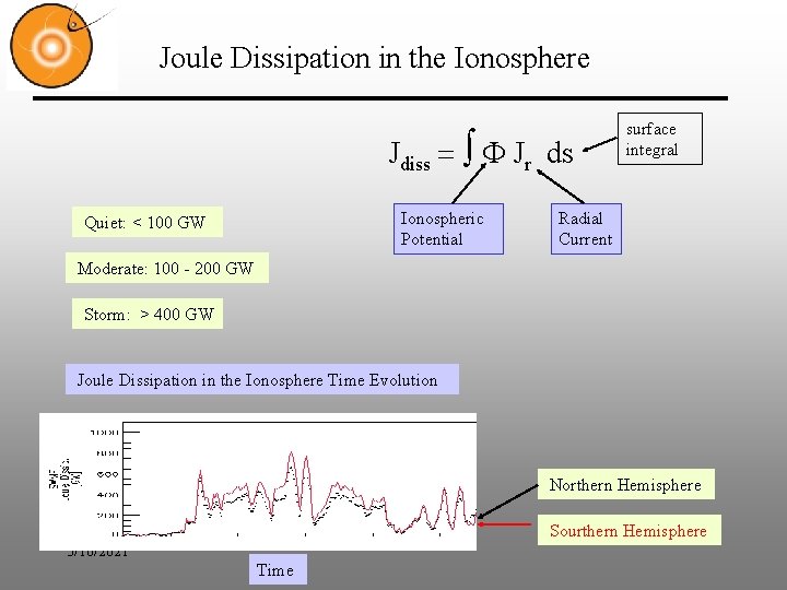
Joule Dissipation in the Ionosphere Jdiss = F Jr ds Ionospheric Potential Quiet: < 100 GW surface integral Radial Current Moderate: 100 - 200 GW Storm: > 400 GW Joule Dissipation in the Ionosphere Time Evolution Northern Hemisphere Sourthern Hemisphere 3/10/2021 Time

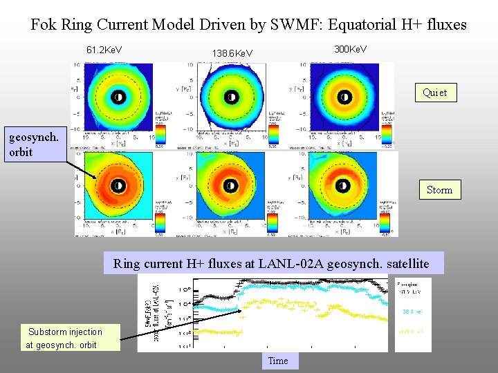
Fok Ring Current Model Driven by SWMF: Equatorial H+ fluxes 61. 2 Ke. V 300 Ke. V 138. 6 Ke. V Quiet geosynch. orbit Storm Ring current H+ fluxes at LANL-02 A geosynch. satellite Substorm injection at geosynch. orbit Time

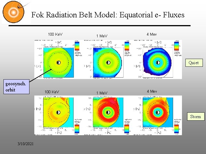
Fok Radiation Belt Model: Equatorial e- Fluxes 100 Ke. V 1 Me. V 4 Mev Quiet geosynch. orbit 100 Ke. V 1 Me. V 4 Mev Storm 3/10/2021

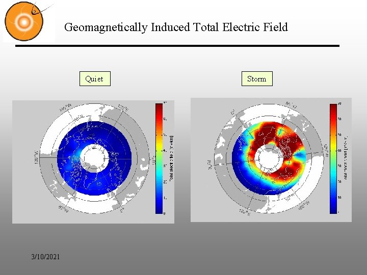
Geomagnetically Induced Total Electric Field Quiet 3/10/2021 Storm

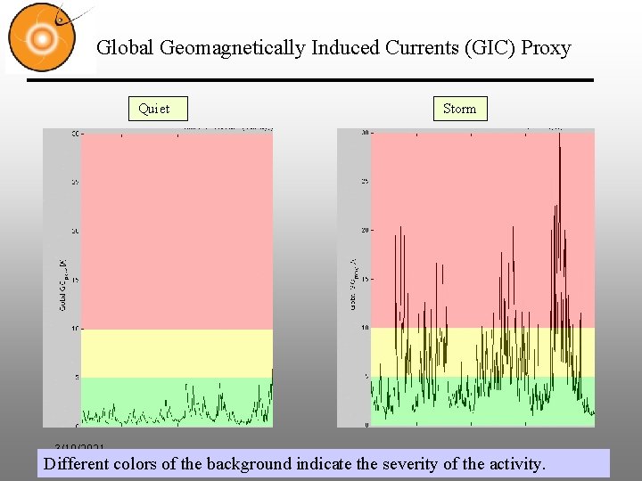
Global Geomagnetically Induced Currents (GIC) Proxy Quiet 3/10/2021 Storm Different colors of the background indicate the severity of the activity.

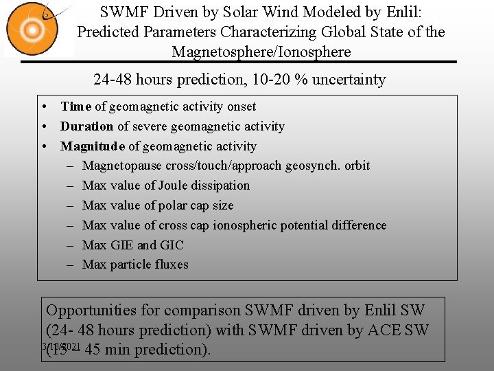
SWMF Driven by Solar Wind Modeled by Enlil: Predicted Parameters Characterizing Global State of the Magnetosphere/Ionosphere 24 -48 hours prediction, 10 -20 % uncertainty • Time of geomagnetic activity onset • Duration of severe geomagnetic activity • Magnitude of geomagnetic activity – Magnetopause cross/touch/approach geosynch. orbit – Max value of Joule dissipation – Max value of polar cap size – Max value of cross cap ionospheric potential difference – Max GIE and GIC – Max particle fluxes Opportunities for comparison SWMF driven by Enlil SW (24 - 48 hours prediction) with SWMF driven by ACE SW 3/10/2021 (15 – 45 min prediction).

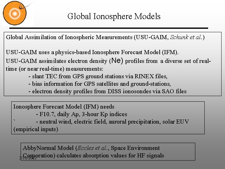
Global Ionosphere Models Global Assimilation of Ionospheric Measurements (USU-GAIM, Schunk et al. ) USU-GAIM uses a physics-based Ionosphere Forecast Model (IFM). USU-GAIM assimilates electron density (Ne) profiles from a diverse set of realtime (or near real-time) measurements: - slant TEC from GPS ground stations via RINEX files, - bias information for GPS satellites and ground-stations, - electron density profiles from DISS ionosondes via SAO files Ionosphere Forecast Model (IFM) needs - F 10. 7, daily Ap, 3 -hour Kp indices ` - neutral wind, electric field, auroral precipitation, solar EUV (empirical inputs) Abby. Normal Model (Eccles et al. , Space Environment Corporation) calculates absorption values for HF signals 3/10/2021

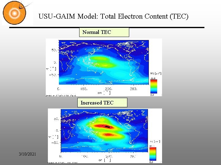
USU-GAIM Model: Total Electron Content (TEC) Normal TEC Increased TEC 3/10/2021

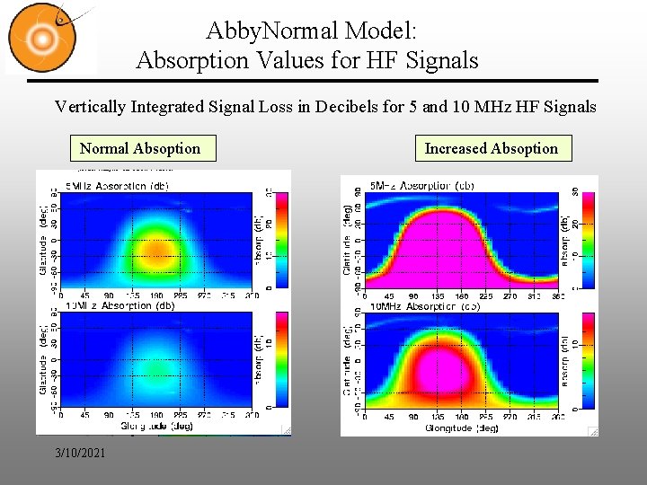
Abby. Normal Model: Absorption Values for HF Signals Vertically Integrated Signal Loss in Decibels for 5 and 10 MHz HF Signals Normal Absoption 3/10/2021 Increased Absoption