Magnetic thin films Physics 201 H from basic

Magnetic thin films: Physics 201 H from basic research to spintronics Christian Binek 11/18/2005 Why thin films Size matters Length (and time) scales determine the physics of a system Quantum mechanics tells us: Confinement of electrons by lowering dimensions affects the electronic states Electronic states 3 D bulk 2 D film 1 D wire 0 D quantum dots artificial atoms all macroscopic properties

Physics 201 H 11/18/2005 When can films considered to be thin or thin with respect to what d d characteristic length Thin in comparison with the characteristic length scale Examples: -Superconducting thin film thickness correlation length -optical thin film like dielectric mirrors Length scale /4 500 nm/4

Physics 201 H -Magnetic thin films approach the ultimate extreme 11/18/2005 thickness quantum mechanical exchange interaction length a few atomic layers Exchange J(d) ferromagnet spacer d nonmagnetic ferromagnet Spacer thickness d in # of atomic layers J(d=8)>0 d=8 monolayer Ferromagnetic coupling J(d=10)<0 d=10 monolayer Antiferromagnetic coupling

How to grow magnetic heterostructures > 250 000 ?

Molecular Beam Epitaxy • Thin film growth @ low deposition rate • Ultra high vacuum condition

Important growth modes in heteroepitaxy specific free energy Layer-by layer (Frank van der Merwe) substrate Monolayer followed by 3 D islands (Stranski Krastanov) deposited material interface 3 D islands (Volmer weber) Reflection High-Energy Electron Diffraction RHEED Electron gun up to 50 ke. V sample RHEED Eye screen camera

What are the magnetic heterolayers good for ? Basic components of modern spintronic devices • Conventional electronics has ignored the spin of the electron • Advantages using spin degree of freedom: magnetic field sensors M-RAM Spin-transistor semiconductor Quantuminformation

• Impact of GMR based field sensors on magnetic data storage Evolution of magnetic data storage on hard disc drives Superparamagnetic effect GMR Magnetoresistive heads inductive read head

rotating sensor layer FM 1 fixed layer FM 2

How to pin FM 2 while the sensor layer FM 1 rotates? Exchange Bias! Pinning of the ferromagnet by an antiferromagnet field cooling: from T>TN to T<TN

Meiklejohn Bean: uniform magnetization reversal of a pinned FM FM interface magnetization: SFM MFM coupling constant: J AF interface magnetization: SAF t. FM KFM, H MFM : saturation magnetization of FM layer Exchange bias field: Stoner-Wohlfarth AF/FM-interface coupling

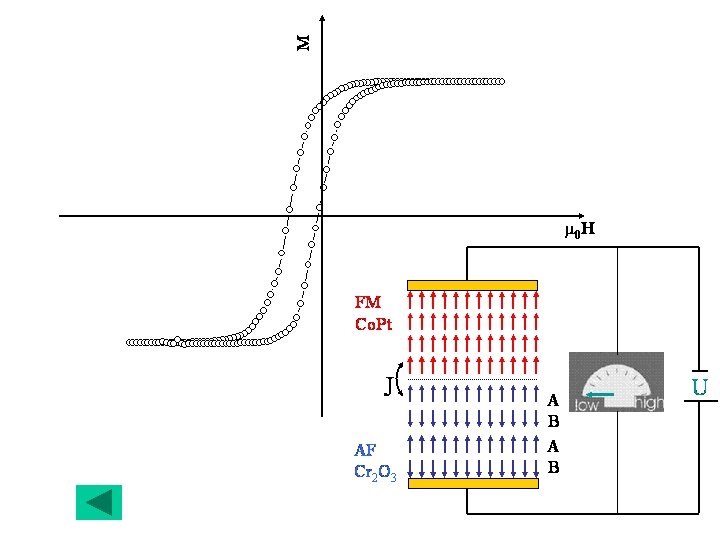
Electric control of the Exchange Bias Investigated multilayer system: Cr 2 O 3(0001)/Pt 0. 67 nm/(Co 0. 35 nm/Pt 1. 2 nm)3/Pt 3. 1 nm t. Pt=1. 20 nm Co Co U Co Pt Pt t. Co=0. 35 nm FM thin film with perpendicular magnetic anisotropy Pt Cr 2 O 3: Magnetoeletric AF, T Magnetoeletric effect of Cr N=308 K 2 O 3 SQUID-magnetometry @ T=290 K * electric field E=U/d Cr 2 O 3 (0001) Idea: E M contributes to SAF Magnetization M=m/V U Cr 2 O 3 (0001) *A. Hochstrat, Ch. Binek, Xi Chen, W. Kleemann, JMMM 272 -276, 325 (2003)

Change of the exchange bias field as a function of the electric field at T = 150 K U=Ed Co Pt Cr 2 O 3 (0001)

2 Magnetoelectric Switching of Exchange Bias*: Control via field-cooling *P. Borisov, A. Hochstrat, Xi Chen, W. Kleemann and Ch. Binek, PRL 94 117203 (2005) Magneto-optical Kerr measurements @ T = 298 K after cooling from T>TN in 0 Hfr = 0. 6 T Magnetic Field Cooling (MFC) (+, -) Efr. Hfr<0 (+, +) Efr. Hfr>0 cooling from M E F C (+, -) T>TN a l i o in 0 Hfr = +0. 6 T g e e o n c l l and e t d i n t r Efr=-500 k. V/m g i o c [T] cooling from M E F C (+, +) T>TN a l i o in 0 Hfr =+0. 6 T g e e o n c l l and e t d i n Efr=+500 k. V/m ot ri g The sign of the Exchange bias follows the sign of Efr. Hfr c

Spintronic applications* *Ch. Binek and B. Doudin, J. Phys. : Condens. Matter 17 (2005) L 39–L 44 V V FM 2 ME ME FM 1 R H

V V FM 2 NM NM FM 1 ME ME R -He-Hi H

Exclusive Or x | y | x. ORy 0 | 0 0 | 1 1 | 0 Example: 0 +V -H X: = Voltage Input Y: = magn. field +V 0 -V 1 +H 1 -H 0 R high 0 R low 1 Output R 0 H

Basic research with magnetic heterostructures generalized Meiklejohn Bean approach finite anisotropy KAF≠ 0 J : coupling constant SAF/FM : AF/FM interface magnetization t. AF/FM : AF/FM layer thickness MFM : saturation magnetization of FM layer Experimental check of advanced models understanding the basic microscopic mechanism of exchange bias Exchange bias is a non-equilibrium phenomenon new approach to relaxation phenomena in non-equilibrium thermodynamics

The training effect: a novel approach to study relaxation physics Training effect: reduction of the EB shift upon subsequent magnetization reversal of the FM layer - origin of training effect - simple expression for

Relaxation towards equilibrium Landau-Khalatnikov : phenomenological damping constant Training not continuous process in time, but triggered by FM loop discretization of the LK- equation Discretization: LK- differential equation difference equation

Comparison with experimental results on Ni. O-Fe 1 st& 9 th hysteresis of Ni. O(001)/Fe (001) compensated 12 nm Fe Ni. O

experimental data recursive sequence min. 0. 015 (m. T)-2 e and e 3. 66 m. T

Magnetic Nanoparticles Collaborations self-assembled Co clusters I thermally decompose You want to know metal carbonyls what I am doing? in the presence of appropriate surfactants Transmission electron microscopic image ~5 nm

Fundamental questions Which magnetic interactions dominate the system What kind of magnetic order can we observe For large particle distances the dipolar interaction will dominate

Here is a real fundamental question: Do dipolar systems still obey extensive thermodynamics What does this mean: Magnetic moment , T, H =2 Magnetic moment Simulations suggest: Yes: for a 2 dimensional array of dipolar interacting particles but No: for a 3 dimensional array of dipolar interacting particles Modifications of conventional thermodynamics required , T, H

Summary MBE is a technology at the forefront of modern material science magnetic heterolayers are basic ingredients for spintronic applications magnetism of thin films and nanoparticles provides experimental access to fundamental questions in statistical physics

Mechanical analogy F( ) V(X) equilibrium xeq Damped harmonic oscillator: x - eq equilibrium eq

Solution for: with

where also derived from integration of: m 0 Temporal evolution of X with increasing damping:

384, 400 km Near earth outer space: