MAE 3241 AERODYNAMICS AND FLIGHT MECHANICS Compressible Flow

MAE 3241: AERODYNAMICS AND FLIGHT MECHANICS Compressible Flow Over Airfoils: Linearized Subsonic Flow Mechanical and Aerospace Engineering Department Florida Institute of Technology D. R. Kirk

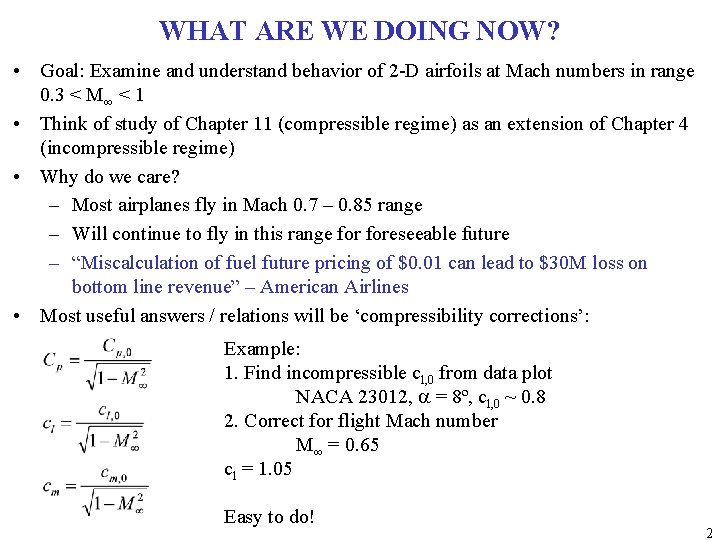
WHAT ARE WE DOING NOW? • Goal: Examine and understand behavior of 2 -D airfoils at Mach numbers in range 0. 3 < M∞ < 1 • Think of study of Chapter 11 (compressible regime) as an extension of Chapter 4 (incompressible regime) • Why do we care? – Most airplanes fly in Mach 0. 7 – 0. 85 range – Will continue to fly in this range foreseeable future – “Miscalculation of fuel future pricing of $0. 01 can lead to $30 M loss on bottom line revenue” – American Airlines • Most useful answers / relations will be ‘compressibility corrections’: Example: 1. Find incompressible cl, 0 from data plot NACA 23012, a = 8º, cl, 0 ~ 0. 8 2. Correct for flight Mach number M∞ = 0. 65 cl = 1. 05 Easy to do! 2

PREVIEW: COMPRESSIBILITY CORRECTION EFFECT OF M∞ ON CP Sound Barrier ? For M∞ < 0. 3, r ~ const Cp = Cp, 0 = 0. 5 = const Effect of compressibility (M∞ > 0. 3) is to increase absolute magnitude of Cp and M∞ increases Called: Prandtl-Glauert Rule M∞ Prandtl-Glauert rule applies for 0. 3 < M∞ < 0. 7 (Why not M∞ = 0. 99? ) 3

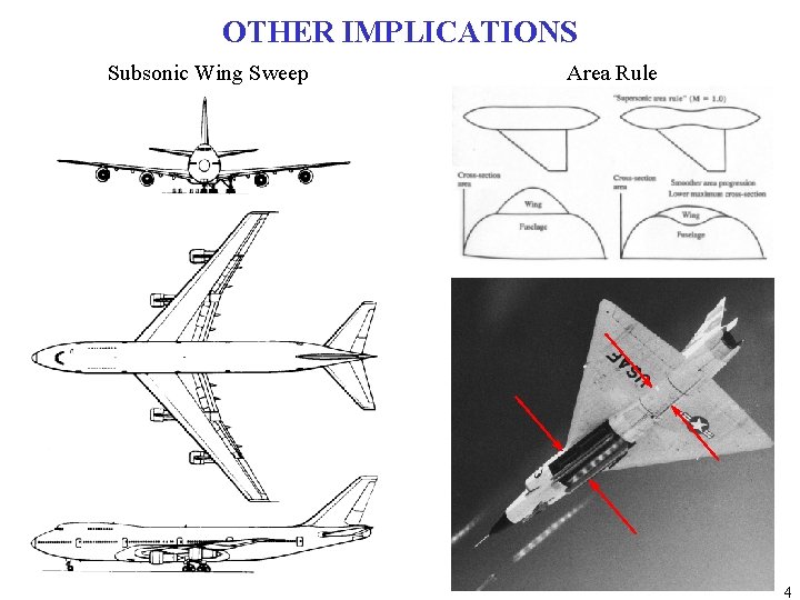
OTHER IMPLICATIONS Subsonic Wing Sweep Area Rule 4

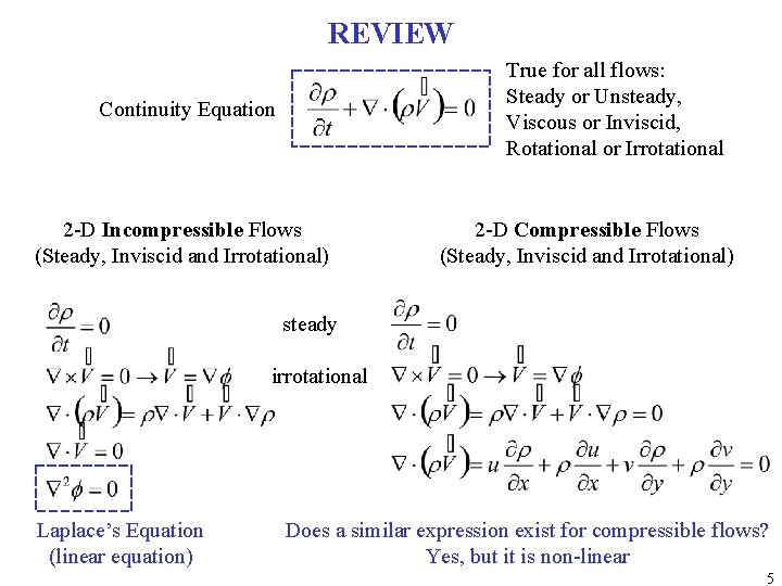
REVIEW True for all flows: Steady or Unsteady, Viscous or Inviscid, Rotational or Irrotational Continuity Equation 2 -D Incompressible Flows (Steady, Inviscid and Irrotational) 2 -D Compressible Flows (Steady, Inviscid and Irrotational) steady irrotational Laplace’s Equation (linear equation) Does a similar expression exist for compressible flows? Yes, but it is non-linear 5

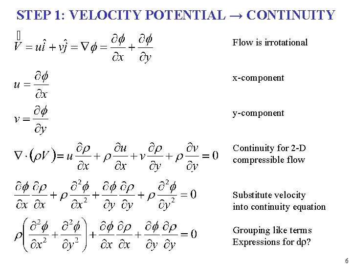
STEP 1: VELOCITY POTENTIAL → CONTINUITY Flow is irrotational x-component y-component Continuity for 2 -D compressible flow Substitute velocity into continuity equation Grouping like terms Expressions for dr? 6

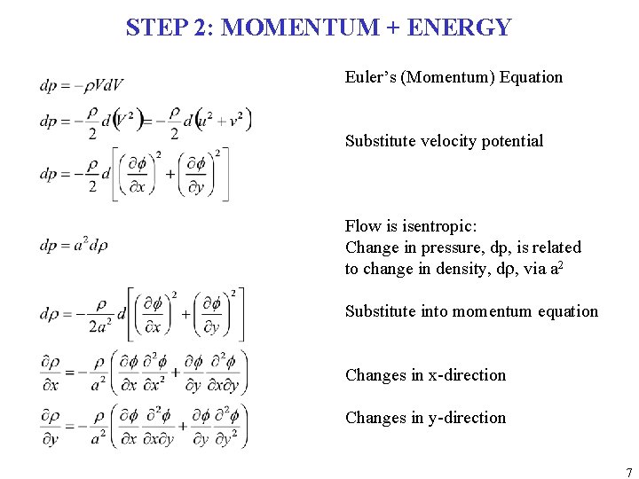
STEP 2: MOMENTUM + ENERGY Euler’s (Momentum) Equation Substitute velocity potential Flow is isentropic: Change in pressure, dp, is related to change in density, dr, via a 2 Substitute into momentum equation Changes in x-direction Changes in y-direction 7

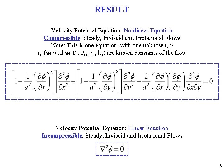
RESULT Velocity Potential Equation: Nonlinear Equation Compressible, Steady, Inviscid and Irrotational Flows Note: This is one equation, with one unknown, f a 0 (as well as T 0, P 0, r 0, h 0) are known constants of the flow Velocity Potential Equation: Linear Equation Incompressible, Steady, Inviscid and Irrotational Flows 8

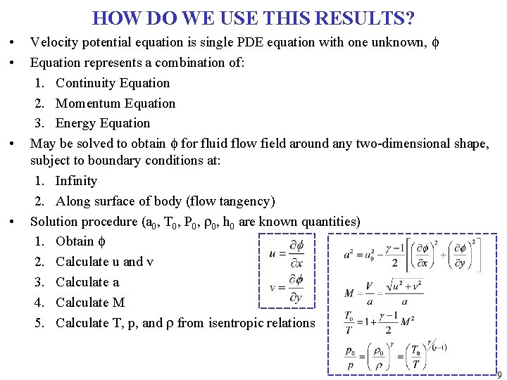
HOW DO WE USE THIS RESULTS? • • Velocity potential equation is single PDE equation with one unknown, f Equation represents a combination of: 1. Continuity Equation 2. Momentum Equation 3. Energy Equation May be solved to obtain f for fluid flow field around any two-dimensional shape, subject to boundary conditions at: 1. Infinity 2. Along surface of body (flow tangency) Solution procedure (a 0, T 0, P 0, r 0, h 0 are known quantities) 1. Obtain f 2. Calculate u and v 3. Calculate a 4. Calculate M 5. Calculate T, p, and r from isentropic relations 9

WHAT DOES THIS MEAN, WHAT DO WE DO NOW? • Linearity: PDE’s are either linear or nonlinear – Linear PDE’s: The dependent variable, f, and all its derivatives appear in a linear fashion, for example they are not multiplied together or squared • No general analytical solution of compressible flow velocity potential is known – Resort to finite-difference numerical techniques • Can we explore this equation for a special set of circumstances where it may simplify to a linear behavior (easy to solve)? 1. Slender bodies 2. Small angles of attack – Both are relevant for many airfoil applications and provide qualitative and quantitative physical insight into subsonic, compressible flow behavior • Next steps: – Introduce perturbation theory (finite and small) – Linearize PDE subject to (1) and (2) and solve for f, u, v, etc. 10

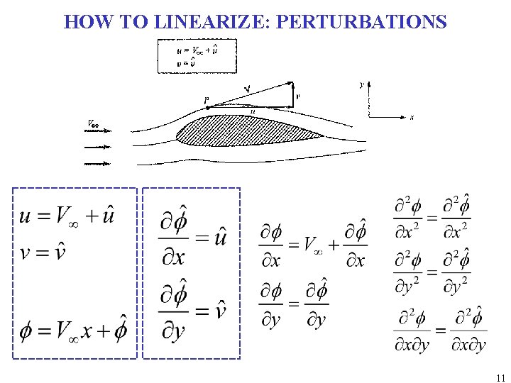
HOW TO LINEARIZE: PERTURBATIONS 11

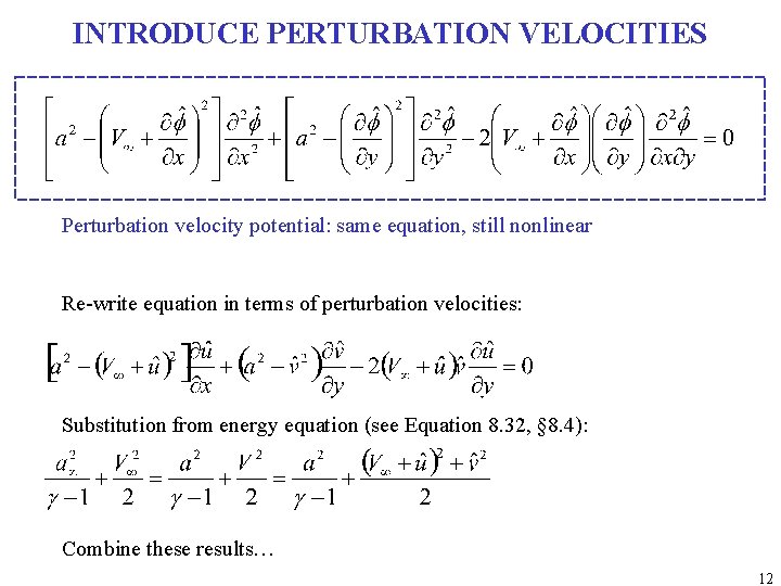
INTRODUCE PERTURBATION VELOCITIES Perturbation velocity potential: same equation, still nonlinear Re-write equation in terms of perturbation velocities: Substitution from energy equation (see Equation 8. 32, § 8. 4): Combine these results… 12

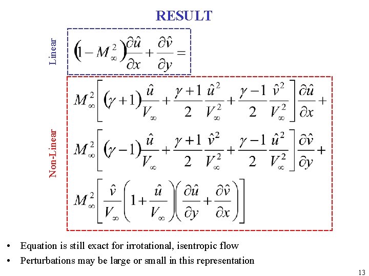
Non-Linear RESULT • Equation is still exact for irrotational, isentropic flow • Perturbations may be large or small in this representation 13

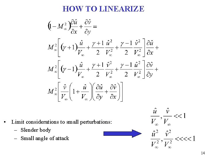
HOW TO LINEARIZE • Limit considerations to small perturbations: – Slender body – Small angle of attack 14

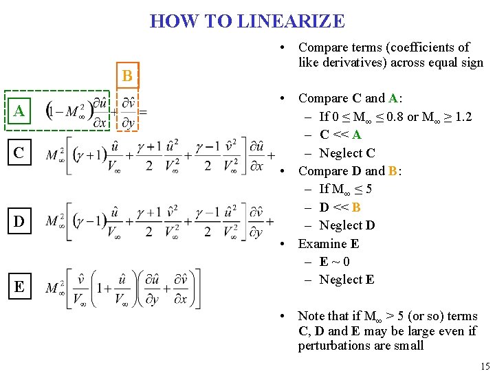
HOW TO LINEARIZE B A C D E • Compare terms (coefficients of like derivatives) across equal sign • Compare C and A: – If 0 ≤ M∞ ≤ 0. 8 or M∞ ≥ 1. 2 – C << A – Neglect C • Compare D and B: – If M∞ ≤ 5 – D << B – Neglect D • Examine E – E~0 – Neglect E • Note that if M∞ > 5 (or so) terms C, D and E may be large even if perturbations are small 15

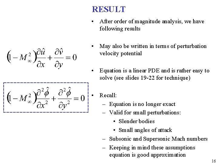
RESULT • After order of magnitude analysis, we have following results • May also be written in terms of perturbation velocity potential • Equation is a linear PDE and is rather easy to solve (see slides 19 -22 for technique) • Recall: – Equation is no longer exact – Valid for small perturbations: • Slender bodies • Small angles of attack – Subsonic and Supersonic Mach numbers – Keeping in mind these assumptions equation is good approximation 16

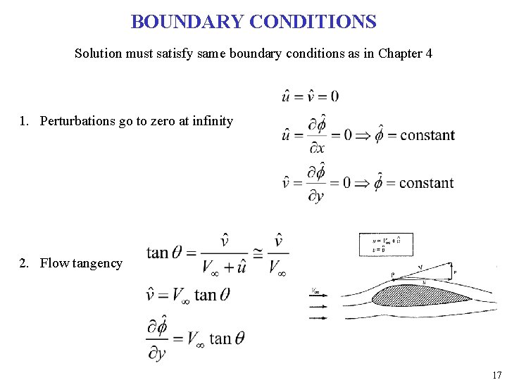
BOUNDARY CONDITIONS Solution must satisfy same boundary conditions as in Chapter 4 1. Perturbations go to zero at infinity 2. Flow tangency 17

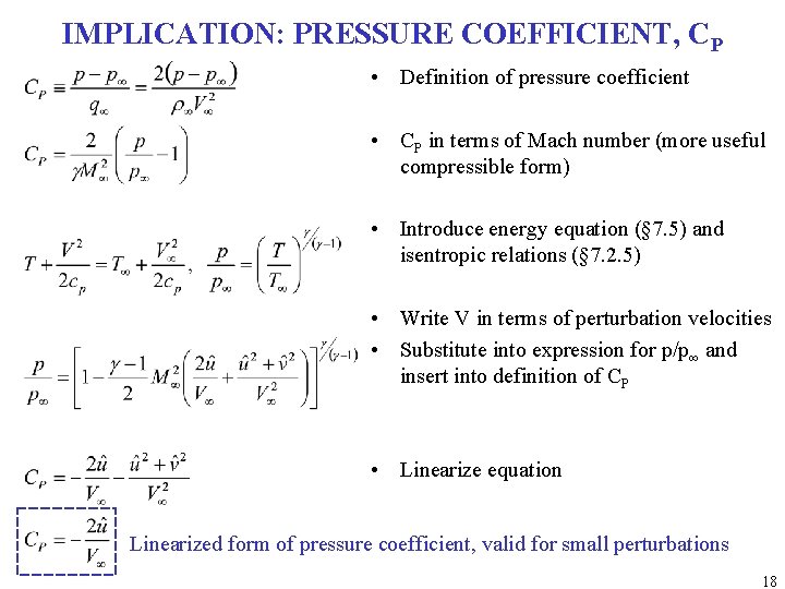
IMPLICATION: PRESSURE COEFFICIENT, CP • Definition of pressure coefficient • CP in terms of Mach number (more useful compressible form) • Introduce energy equation (§ 7. 5) and isentropic relations (§ 7. 2. 5) • Write V in terms of perturbation velocities • Substitute into expression for p/p∞ and insert into definition of CP • Linearize equation Linearized form of pressure coefficient, valid for small perturbations 18

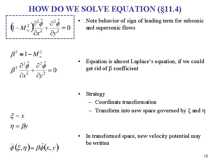
HOW DO WE SOLVE EQUATION (§ 11. 4) • Note behavior of sign of leading term for subsonic and supersonic flows • Equation is almost Laplace’s equation, if we could get rid of b coefficient • Strategy – Coordinate transformation – Transform into new space governed by x and h • In transformed space, new velocity potential may be written 19

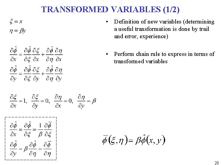
TRANSFORMED VARIABLES (1/2) • Definition of new variables (determining a useful transformation is done by trail and error, experience) • Perform chain rule to express in terms of transformed variables 20

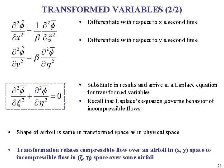
TRANSFORMED VARIABLES (2/2) • Differentiate with respect to x a second time • Differentiate with respect to y a second time • Substitute in results and arrive at a Laplace equation for transformed variables • Recall that Laplace’s equation governs behavior of incompressible flows • Shape of airfoil is same in transformed space as in physical space • Transformation relates compressible flow over an airfoil in (x, y) space to incompressible flow in (x, h) space over same airfoil 21

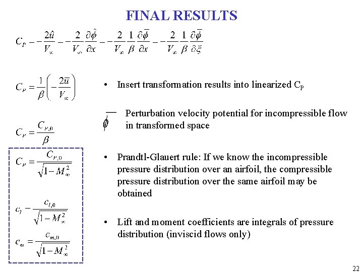
FINAL RESULTS • Insert transformation results into linearized CP Perturbation velocity potential for incompressible flow in transformed space • Prandtl-Glauert rule: If we know the incompressible pressure distribution over an airfoil, the compressible pressure distribution over the same airfoil may be obtained • Lift and moment coefficients are integrals of pressure distribution (inviscid flows only) 22

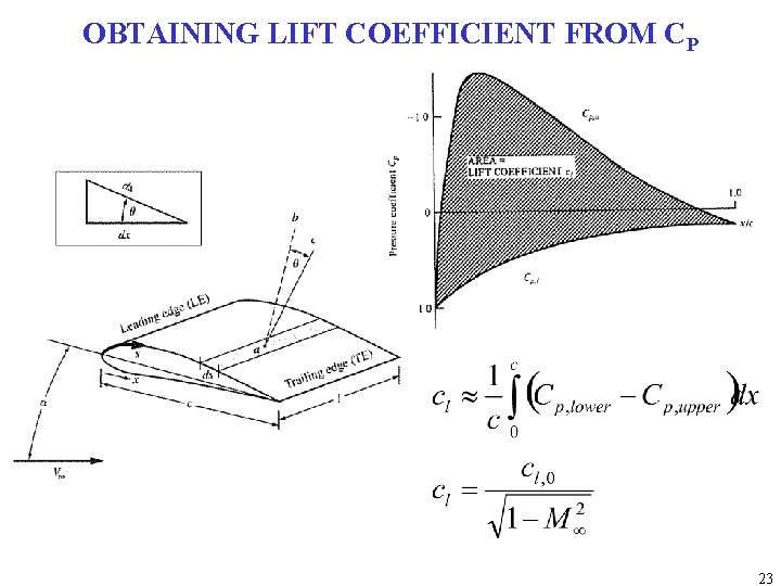
OBTAINING LIFT COEFFICIENT FROM CP 23

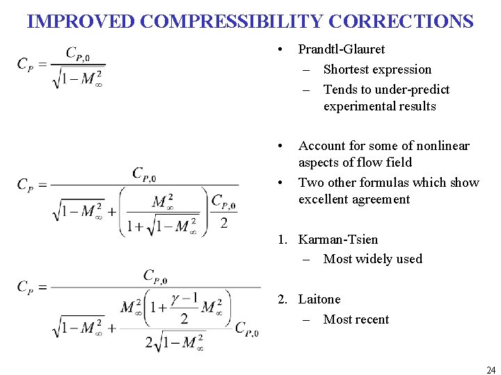
IMPROVED COMPRESSIBILITY CORRECTIONS • Prandtl-Glauret – Shortest expression – Tends to under-predict experimental results • Account for some of nonlinear aspects of flow field Two other formulas which show excellent agreement • 1. Karman-Tsien – Most widely used 2. Laitone – Most recent 24