Macroscopic Flow Characteristics Temporal Flow Patterns Spatial Flow

Macroscopic Flow Characteristics • Temporal Flow Patterns • Spatial Flow Patterns • Modal Flow Patterns

Introduction • Traffic flow represents the traffic load on the transportation system and the interaction between these loadings, and the facility capacity determines the operational performance of the system. It is extremely important, therefore to know the flow rates, their temporal, spatial and modal variations, and the composition of the traffic stream. • Macroscopic flow characteristics important for – Planning – Design – Operation and management

Macroscopic Flow Terms • Flow Rate is defined as the number of vehicles passing a point in a given period of time (often less than one hour), and is expressed as an hourly flow rate. Because of the variation in the flow rate over time, not only does the flow rate need to be defined, but also the period of time over which the flow rate was measured. • Four important flow parameters – – Demand Service volume Capacity Saturation flow rate

Demand • Existing traffic demand is the flow rate value used to analyze an oversaturated or congested condition, and represents the flow rate at which vehicles would like to be serviced. • The existing traffic demand is equal to the measured flow rate if there is no over saturation upstream or congestion at the point in question. • If over saturation or congestion is encountered, the flow rate is indicative only of the flow rate level that can be handled, and is not an indication of the existing traffic demand.

Volume • Volume: number of units that are actually being served per unit time • Volume is typically defined for one hour or longer • (max) Service flow rate (volume) is defined as the maximum hourly rate at which persons or vehicles can reasonably be expected to traverse a point during a given interval of time (15 minutes) under prevailing roadway, traffic and control conditions while maintaining a designated level of service (except LOS F).

Service Flow Rate Service flow rate for LOS E: capacity – e. g. , If actual flow> (max) service flow rate for LOS B & < (max) service flow rate for LOS C == > LOS is C

Capacity • Capacity is defined as the maximum hourly rate at which persons or vehicles can reasonably be expected to traverse a point during a given interval of time (15 minutes) under prevailing roadway, traffic and control conditions.

Saturation flow rate • Saturation flow rate is defined as the equivalent maximum hourly rate at which vehicles can traverse a lane under prevailing traffic and roadway conditions assuming that the green signal is available at all times, and no loss times are experienced. • Saturation flow rate is a term for interrupted flow.

Input – Output Analysis System Defined Must have knowledge of number of vehicles in system at all times

Demand Volume Input-Output Analysis No. of veh in system t 0 t 1 D > V t 0 – t 1 Congestion t 0 – t 2 t St t 0 t 1

Input = Demand Output = Volumes Input-Output Analysis A 1 Capacity A 2 No. of veh in system A 1 = Storage t A 2 = Dissipation Ss So t t 0 t t 1 t 2 Area = System travel time between t 0 & t 2 (time in the system: veh. Hours)

Input-Output Analysis T Cumulative No. of Vehicles Demand N Capacity t 0 t t 2 N = No. of vehicles backed up at time t T = Delay for driver arriving at time t

Flow Rate vs. Volume • Flow: defined as rate for a period shorter than 1 hour • Volume: typically defined over a time that is one hour or longer. E. g. , hourly volume, daily volume, etc. • Peak hour flow rate is used for design and operational analysis. • In the past only “volume” is used

Temporal Flow Patterns • Traffic flow rates vary over time – – Monthly Daily Hourly within-hour variations • It is very important to understand these temporal flow patterns in order to estimate traffic flow rates for selected periods of time based on known flow rates from other periods of time

Temporal Flow Patterns

Temporal Flow Patterns

Temporal Flow Patterns

Temporal Flow Patterns

Temporal Flow Patterns Data from Houston

Temporal Flow Patterns Data from Houston (two directions combined)

Temporal Flow Patterns Speed changes due to daily temporal flow pattern

Spatial Flow Patterns • Traffic flow rates vary over space, and consequently, linear, network, directional and lane use variations are important concepts.

Linear Flow Patterns • Traffic flows can be thought of as waves, and the higher-intensity traffic flows move toward the CBD, resulting in a linear traffic demand pattern. • The inbound peak periods are experienced first on the outskirts of the city, and as time passes, the inbound peak periods move toward the CBD.

Network Flow Patterns • Most highway facilities are connected to dense networks of other facilities. Since motorists have the freedom of choice, and are guided by following the route of least resistance (travel time), there are strong interactions between parallel routes. • As higher-quality routes become oversaturated, motorists divert to parallel lower-quality routes

Directional Flow Patterns • Directional flow pattern exists along some specific routes. • The directional splits during the am and pm peak periods are quite different on most highway types.

Directional Flow Patterns

Lane Use Flow Patterns • The distribution of traffic among lanes varies when more than one lane is available for each direction. • As the total directional flow increases, the percentage of traffic in the median lane typically increases while the percentage of traffic in the shoulder lane decreases.

Lane Use Flow Patterns

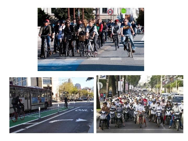
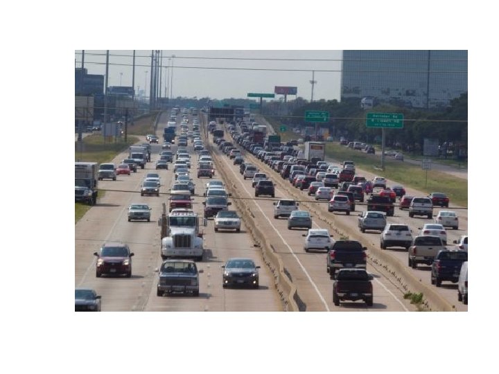
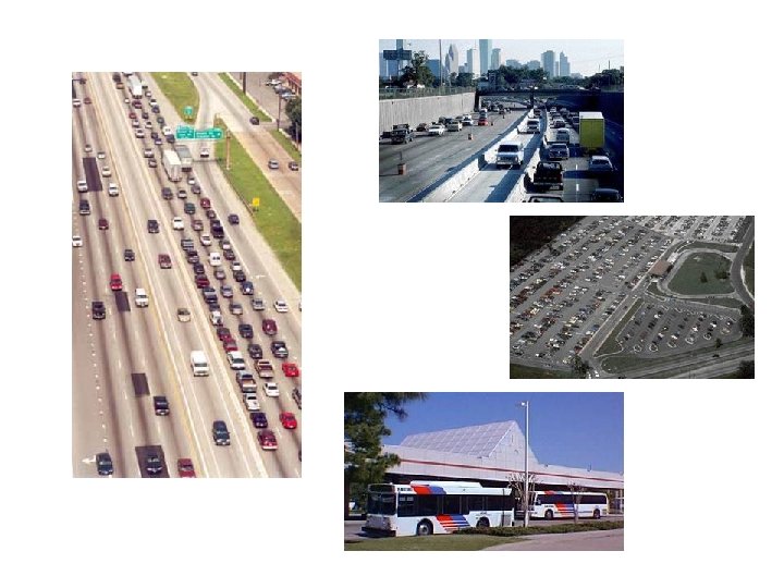
Modal Flow Patterns • Transportation modes involve the distribution of truck, bus, train and passenger car transport. • Modal choice is an important concept because of the widely varying vehicle occupancies and operating characteristics of the vehicle types.

Modal Flow Patterns

Modal Flow Patterns Zhang et al. , 2006

Modal Flow Patterns Zhang et al. , 2006

Effect of Heavy Vehicles on Flow • The presence of large and low-performance vehicles in traffic stream affects the capacity of highway capacity • The passenger car equivalent is representative of the additional space each of the larger vehicles occupy on the highway because of poorer operating characteristics (acceleration, maintenance of velocity on grade and deceleration)

Modal Flow Patterns

Vehicle Occupancy by Mode

Macro Flow vs. Micro. Flow • q: flow rate (vph) • h: average headway (sec/veh)

Volume Planning Volume: ADT or AADT • Daily volume (24 hour average) • Collected at permanent count stations • Not lane or direction specific

Design Hourly Volume (DHV) Hourly (Design) Volume • Demand over one hour period • May be measured by direction • Uses of hourly volumes – Design: geometric features – Operations: performance of facility

Determination of DHV • 30 th highest hourly volume in a year (30 HV) • Estimated from AADT • Collect data on a typical peak hour

30 HV

AADT vs. DHV & DDHV DHV: Design Hourly Volume=Peak Hour Volume K: about. 10 for urban and. 15 for rural DDHV (Directional Design Hourly Volume) D: directional split 0. 5 - 0. 75

K, D Adjustments KD factors can change the numbers completely

K-Factor and D-Factor （Source: Roess, Prassas, and Mc. Sahne, 2004）

Sample Data on SH 6 (Source: Tx. DOT, 2003)

Peak Hour Volume and Flow Rate PHV Highest hourly volume (“Rush hour” volume) Peak hour flow rate • Based on counts within peak hour, less than one hour in length • Units of Measurement: Equivalent Hourly Volume • Example: 1000 vehicles x 60 minutes = 4000 vehicles per hour 15 minutes 1 hour

Peak Hour Factor • Ratio of total hourly volume to the maximum 15 minute flow rate • Equation: where PHF = the Peak Hour Factor V = the Hourly volume, in vph V 15 = the volume during the peak 15 minutes of the peak hour, in veh/15 min • PHF converts SUB-HOURLY peak flow rates to equivalent hourly flow rates

Mathematical Count Distribution • Poisson count distribution for random events (low flow conditions) where x = number of arrivals during specified time interval, m = average arrival rate for the specified interval of time, and e = exponential constant, 2. 71828182

Poisson Distribution Nomograph

Limitations of Poisson Distribution • Appropriate for describing: – Discrete random events – Light traffic with no disturbing factors such as signals • Not suitable when: – Traffic becomes congested – With cyclic disturbance (such as result of signals) – Mean and variance are significantly different

Other Count Distributions • Binomial Distribution – Congested traffic – Ratio of observed variance/mean substantially less than 1 • Negative Binomial Distribution – High variance from factors such as varying flow rate, upstream/downstream signals, etc. – Ratio of observed variance/mean substantially greater than 1

Binomial Distribution • p is the probability that one car arrives • Cnx is the combination of n things taken x at a time • Mean m=np • Variance s 2=np(1 -p)

Negative Binomial Distribution • Also called Pascal distribution

Summary of Elementary Counting Distributions • Poisson dist. represents the random occurrence of discrete events • In counts of light traffic where the observed data produce a ratio of variance to mean of approximately 1. 0, the Poisson dist. may be fitted to the observed data. • In counts of congested traffic flow where the observed data produce a ratio of variance to mean of substantially less than 1. 0, the binomial dist. may be fitted to the observed data • In counts of traffic where there is a cyclic variation in the flow or where the mean flow is changing during the counting period, giving a ratio of variance to mean substantially greater than 1. 0, the negative binomial dist. may be fitted to the observed data

Capacity of Uninterrupted Flow Facilities