Macroeconomics Module 8 The Aggregate DemandAggregate Supply Model

Macroeconomics Module 8: The Aggregate Demand-Aggregate Supply Model

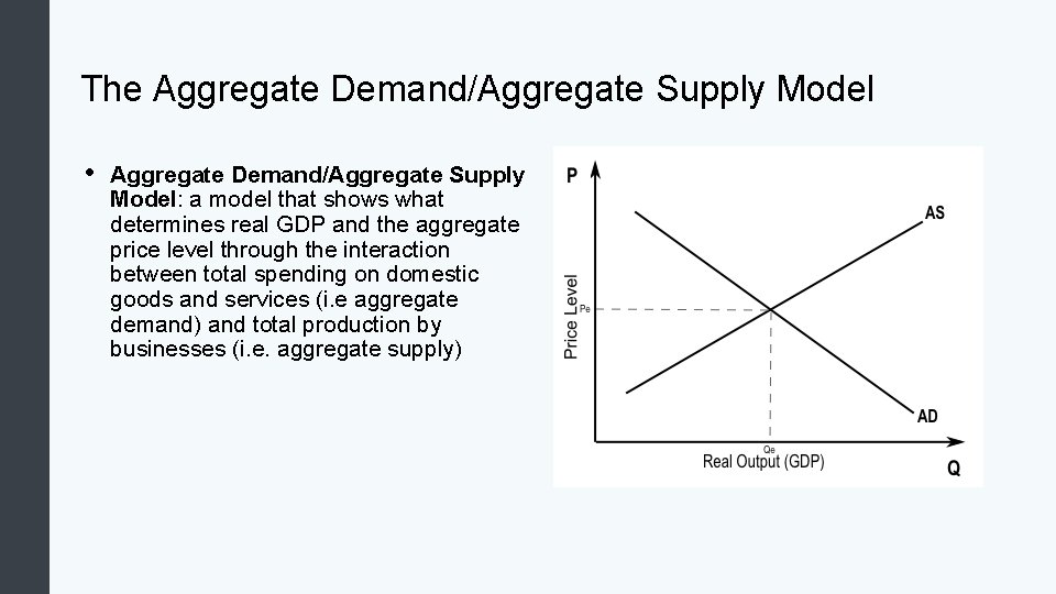
The Aggregate Demand/Aggregate Supply Model • Aggregate Demand/Aggregate Supply Model: a model that shows what determines real GDP and the aggregate price level through the interaction between total spending on domestic goods and services (i. e aggregate demand) and total production by businesses (i. e. aggregate supply)

Building a Model of Aggregate Supply and Aggregate Demand Vocabulary • • • Aggregate Demand (AD): the amount of total spending on domestic goods and services in an economy Aggregate Supply (AS): the total quantity of output (ie real GDP) firms will produce and sell Aggregate Demand (AD) curve: the total spending on domestic goods and services at each aggregate price level Aggregate Supply (AS) curve: the total quantity of output (ie real GDP) that firms will produce and sell at each aggregate price level Foreign Price Effect: if prices rise in the United States while remaining fixed in other countries, then goods in the United States will be relatively more expensive compared to goods in the rest of the world Interest Rate Effect: as the aggregate price level rises, the same purchases will take more money or credit to accomplish, driving up interest rates

Building a Model of Aggregate Supply and Aggregate Demand Vocabulary (cont. ) • • • Long Run: period of time during which all wages and prices are fully flexible Long Run Aggregate Supply (LRAS) curve: vertical line at potential GDP showing no relationship between the aggregate price level and real GDP in the long run Potential GDP: the maximum quantity that an economy can produce given full employment of its existing levels of labor, physical capital, technology, and institutions; also known as full employment GDP Short Run: period of time during which wages (and some prices) are sticky in response to a change in demand Short Run Aggregate Supply (SRAS) curve: positive short run relationship between the aggregate price level and real GDP, holding the prices of inputs fixed Wealth Effect: as price level increases, the buying power of savings that people have stored up in bank accounts and other assets will diminish

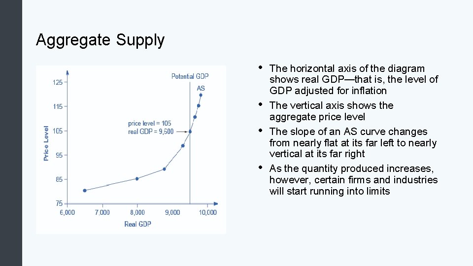
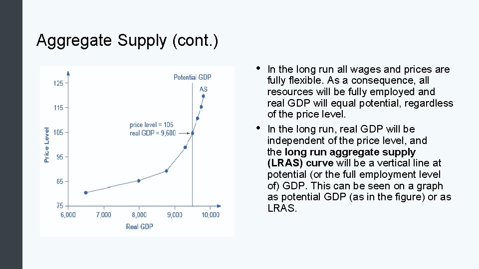
Aggregate Supply • • The horizontal axis of the diagram shows real GDP—that is, the level of GDP adjusted for inflation The vertical axis shows the aggregate price level The slope of an AS curve changes from nearly flat at its far left to nearly vertical at its far right As the quantity produced increases, however, certain firms and industries will start running into limits

Aggregate Supply (cont. ) • • In the long run all wages and prices are fully flexible. As a consequence, all resources will be fully employed and real GDP will equal potential, regardless of the price level. In the long run, real GDP will be independent of the price level, and the long run aggregate supply (LRAS) curve will be a vertical line at potential (or the full employment level of) GDP. This can be seen on a graph as potential GDP (as in the figure) or as LRAS.

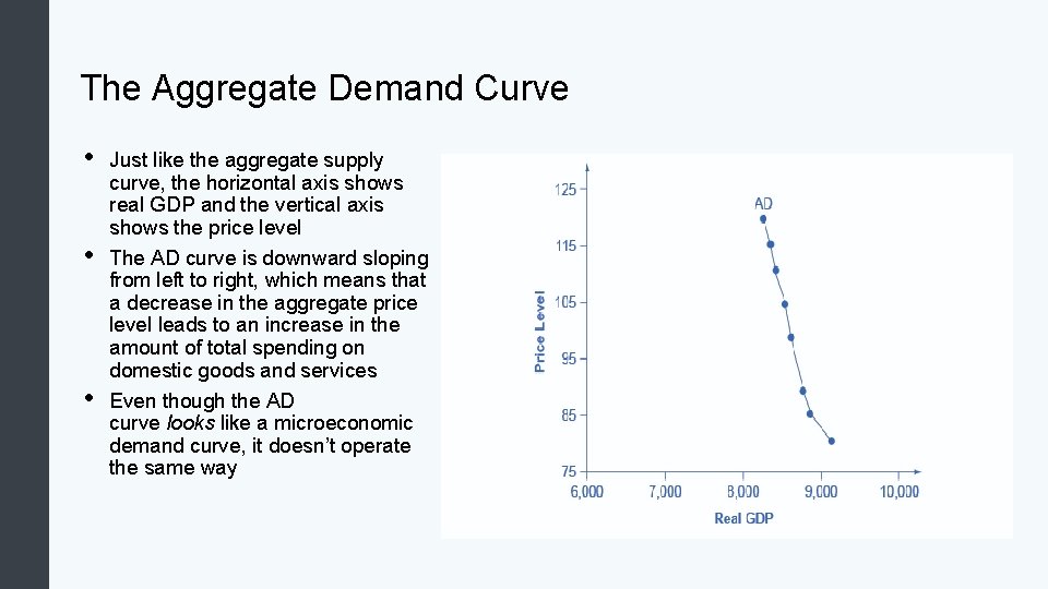
The Aggregate Demand Curve • • • Just like the aggregate supply curve, the horizontal axis shows real GDP and the vertical axis shows the price level The AD curve is downward sloping from left to right, which means that a decrease in the aggregate price level leads to an increase in the amount of total spending on domestic goods and services Even though the AD curve looks like a microeconomic demand curve, it doesn’t operate the same way

Why is the AD Curve downward-sloping? • • • Wealth effect: as the price level increases, the buying power of savings that people have saved up will diminish, eaten away to some extent by inflation. Because a rise in the price level reduces people’s wealth, consumption spending will fall as the price level rises. Interest rate effect: as prices for outputs rise, the same purchases will take more money or credit to accomplish. This additional demand for money and credit will push interest rates higher, which will reduce borrowing by businesses for investment purposes and reduce borrowing by households for homes and cars—thus reducing consumption and investment spending. Foreign price effect: if prices rise in the United States while remaining fixed in other countries, then goods in the United States will be relatively more expensive compared to goods in the rest of the world. A higher domestic price level, relative to price levels in other countries, will reduce net export expenditures.

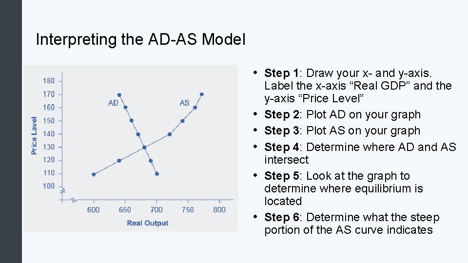
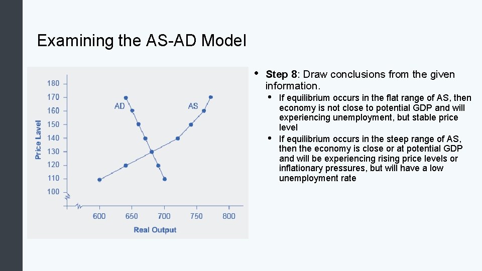
Interpreting the AD-AS Model • Step 1: Draw your x- and y-axis. • • • Label the x-axis “Real GDP” and the y-axis “Price Level” Step 2: Plot AD on your graph Step 3: Plot AS on your graph Step 4: Determine where AD and AS intersect Step 5: Look at the graph to determine where equilibrium is located Step 6: Determine what the steep portion of the AS curve indicates

Examining the AS-AD Model • Step 8: Draw conclusions from the given information. • • If equilibrium occurs in the flat range of AS, then economy is not close to potential GDP and will experiencing unemployment, but stable price level If equilibrium occurs in the steep range of AS, then the economy is close or at potential GDP and will be experiencing rising price levels or inflationary pressures, but will have a low unemployment rate

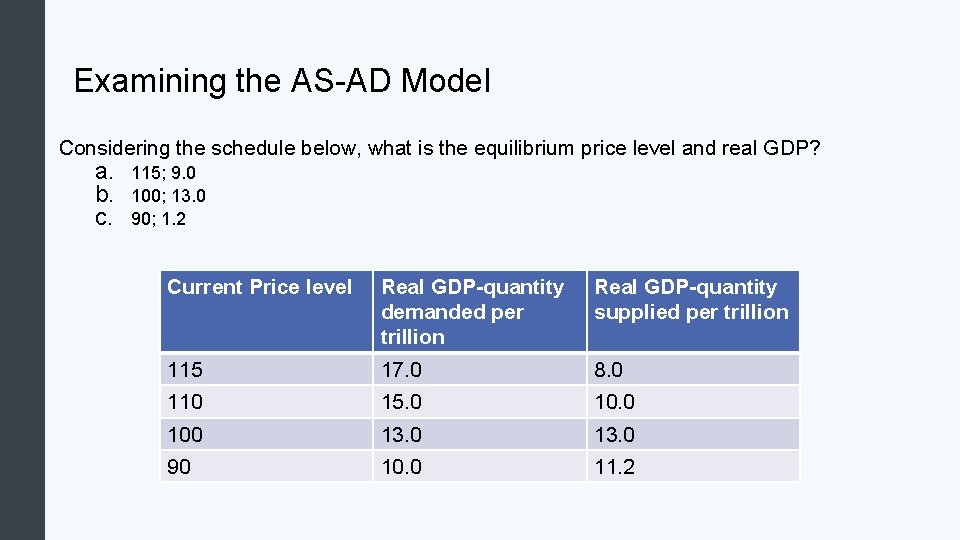
Examining the AS-AD Model Considering the schedule below, what is the equilibrium price level and real GDP? a. b. c. 115; 9. 0 100; 13. 0 90; 1. 2 Current Price level Real GDP-quantity demanded per trillion Real GDP-quantity supplied per trillion 115 17. 0 8. 0 110 15. 0 100 13. 0 90 10. 0 11. 2

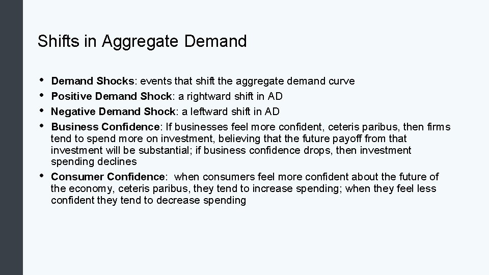
Shifts in Aggregate Demand • • • Demand Shocks: events that shift the aggregate demand curve Positive Demand Shock: a rightward shift in AD Negative Demand Shock: a leftward shift in AD Business Confidence: If businesses feel more confident, ceteris paribus, then firms tend to spend more on investment, believing that the future payoff from that investment will be substantial; if business confidence drops, then investment spending declines Consumer Confidence: when consumers feel more confident about the future of the economy, ceteris paribus, they tend to increase spending; when they feel less confident they tend to decrease spending

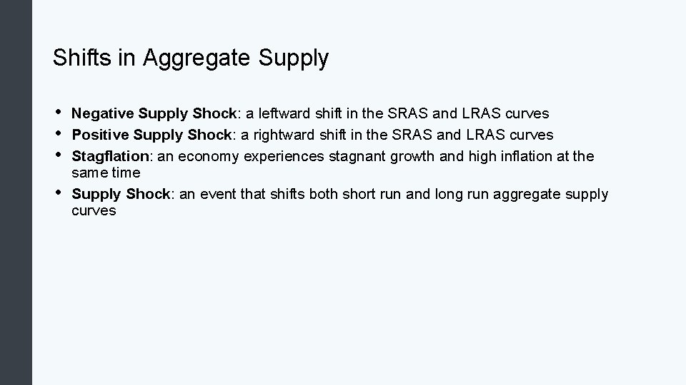
Shifts in Aggregate Supply • • Negative Supply Shock: a leftward shift in the SRAS and LRAS curves Positive Supply Shock: a rightward shift in the SRAS and LRAS curves Stagflation: an economy experiences stagnant growth and high inflation at the same time Supply Shock: an event that shifts both short run and long run aggregate supply curves

Shifts in AD OR AS? When an economy’s output increases and the price level increases, the ____ curve has shifted to the ____. a. b. c. AS; left AD; right

How Productivity Growth Shifts the AS Curve • • • The most important factor shifting the AS curve is productivity growth Productivity means how much output can be produced with a given quantity of inputs Productivity grows so that the same quantity of labor can produce more output The real growth in GDP per capita in an advanced economy like the United States has averaged about 2% to 3% per year Productivity growth has been faster during certain extended periods like the 1960 s and the late 1990 s through the early 2000 s, or slower during periods like the 1970 s

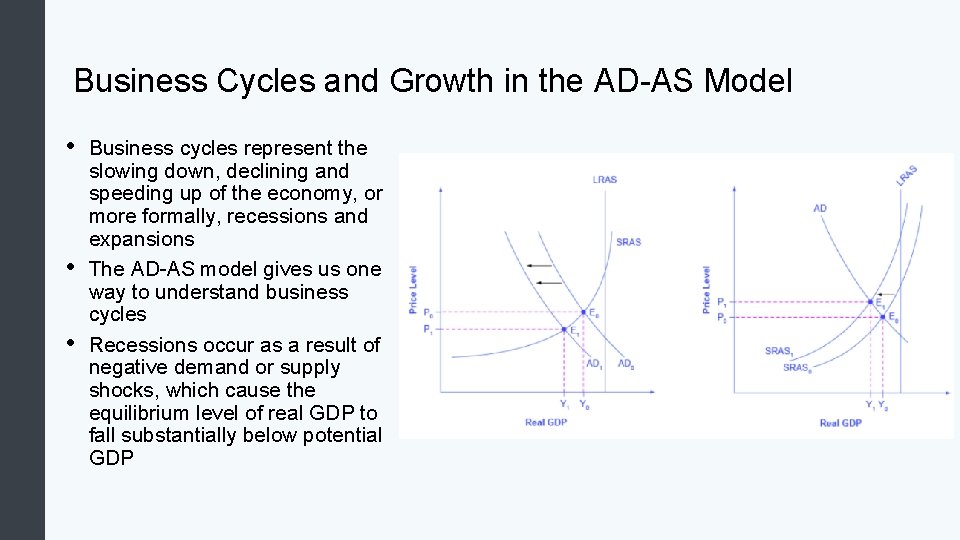
Business Cycles and Growth in the AD-AS Model • • • Business cycles represent the slowing down, declining and speeding up of the economy, or more formally, recessions and expansions The AD-AS model gives us one way to understand business cycles Recessions occur as a result of negative demand or supply shocks, which cause the equilibrium level of real GDP to fall substantially below potential GDP

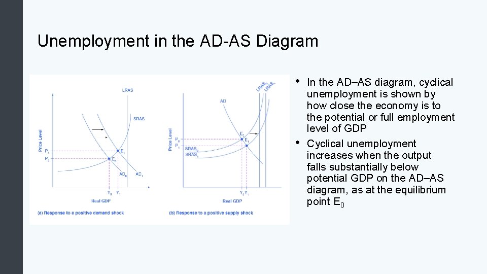
Unemployment in the AD-AS Diagram • • In the AD–AS diagram, cyclical unemployment is shown by how close the economy is to the potential or full employment level of GDP Cyclical unemployment increases when the output falls substantially below potential GDP on the AD–AS diagram, as at the equilibrium point E 0

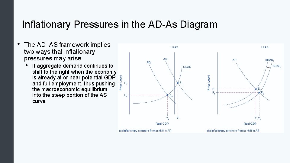
Inflationary Pressures in the AD-As Diagram • The AD–AS framework implies two ways that inflationary pressures may arise • If aggregate demand continues to shift to the right when the economy is already at or near potential GDP and full employment, thus pushing the macroeconomic equilibrium into the steep portion of the AS curve

Quick Review • • Describe the aggregate supply-aggregate demand model Define and explain the aggregate supply curve and the economic behavior behind it Compare and contrast the short run and long run aggregate supply curves Define and explain the aggregate demand curve and the economic behavior behind it What is the difference between the two concepts of aggregate demand aggregate supply? Identify the equilibrium level of real GDP and equilibrium price level using the AD-AS model What conclusions can be made about the macro economy using the AD-AS supply model?

More Quick Review • • • What are the causes and implications of shifts in aggregate demand? How does productivity growth and changes in input prices change the aggregate supply curve? Use the aggregate demand-aggregate supply model to explain recessions, expansions and economic growth Explain how unemployment and inflation can be explained using the aggregate demand-aggregate supply model What is the importance of the AS-AD model?