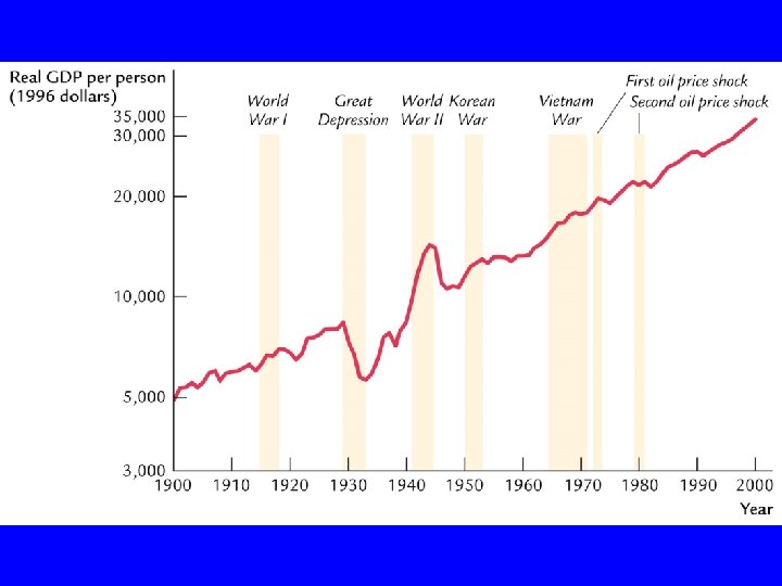
MACROECONOMIC MODELS u Business Cycles Business cycles are

MACROECONOMIC MODELS u Business Cycles – Business cycles are 2 -year to 5 -year fluctuations around trends in real GDP and other related variables

MACROECONOMIC MODELS u Business Cycles – A recession is a large fall in the growth of real GDP and related variables » A depression is an especially large recession
 u Trough u Recovery u")
What Is a Business Cycle? Peak u Contraction (Recession) u Trough u Recovery u Expansion u

Exhibit 7 The Phases of the Business Cycle
 u people are willing")
AGGREGATE DEMAND CURVE shows the amount of real output (RGDP) u people are willing and able to buy u at different price levels u ceteris paribus u
 P 1 A Aggregate Demand")
Aggregate Demand Curve Exhibit 1 Price Level (P ) P 1 A Aggregate Demand Curve The price level and quantity demanded of Real GDP are inversely related. B P 2 AD 0 Q 1 Q 2 Real GDP (Q)

Why Does the Aggregate Demand Curve Slope Downward? Real balance effect u Interest rate effect u International trade effect u

Why Does the Aggregate Demand Curve Slope Downward? u Real balance effect - the purchasing power of a given amount of money buys less at higher price levels than at lower price levels.

REAL BALANCE EFFECT P P 1 Real Balance Effect Price level rises ® purchasing power falls ® monetary wealth falls ® buy fewer goods. Price level falls ® purchasing power rises ® monetary wealth rises ® buy more goods. 2 1 P 2 AD Q 0 P P 1 P 2 1 2 AD 0 Q

Why Does the Aggregate Demand Curve Slope Downward? Real balance effect u Interest rate effect - as price level rises, interest rates tend to rise and the cost of borrowing increases. Int. rate sensitive C and I decrease. u

Interest Rate Effect Price level falls®purchasing power rises®less money needed to buy fixed bundle of goods®save more®supply of credit rises®interest rate falls®businesses and households borrow more at lower interest rate®buy more goods. Price level rises®purchasing power falls®borrow money in order to continue to buy fixed bundle of goods®demand for credit rises®interest rate rises®businesses and households borrow less at higher interest rate®buy fewer goods.

Why Does the Aggregate Demand Curve Slope Downward? Real balance effect u Interest rate effect u International trade effect- as domestic prices rise, imports become cheaper and rise. Exports fall as prices rise. u

INT. TRADE EFFECT P International Trade Effect P 2 Price level in U. S. rises relative to foreign price levels ® U. S. goods relatively more expensive than foreign goods ® both Americans and foreigners buy fewer U. S. goods. P 1 Price level in U. S. falls relative to foreign price levels ® U. S. goods relatively less expensive than foreign goods ® both Americans and foreigners buy more U. S. goods. 2 1 AD 0 Q P P 1 P 2 1 2 AD 0 Q

Changes in the Price level lead to movements along the aggregate demand curve u people buy a higher level of real output at lower price levels u
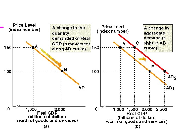

AGGREGATE DEMAND Aggregate demand changes if there is a change in u Total Expenditures u

TOTAL EXPENDITURES change when there are changes in: Consumption u Investment u Government Expenditures u NX=EX - IM u

Exhibit 4 Changes in Aggregate Demand

FACTORS THAT CHANGE CONSUMPTION Wealth u Expectations about future prices and income u Interest rate u Taxes u

FACTORS THAT CHANGE INVESTMENT Interest rate u Expectations about future sales u Business Taxes u

FACTORS THAT CHANGE EX - IM Foreign real national income u Exchange rate u

GOVERNMENT SPENDING Specifics of government spending will be covered in Chapter 8

Exhibit 5 Factors That Change Aggregate Demand
 u shows the amount of")
AGGREGATE SUPPLY The Short Run Aggregate Supply Curve (SRAS) u shows the amount of real output (RGDP) u producers will offer for sale at different price levels u
 SRAS P P 0 B")
Short Run Aggregate Supply Curve Price Level (P ) SRAS P P 0 B Short-Run Aggregate Supply Curve The price level and quantity supplied of Real GDP are directly related. A Q 1 Q 2 Real GDP (Q)

FACTOR THAT SHIFT AGGREGATE SUPPLY The wage rate u prices of nonlabor inputs u productivity u supply shocks u

SUPPLY SHOCKS u ADVERSE – bad weather – cutback in oil – regulatory change u BENEFICIAL – unusually good weather – discovery of a major new resource

Wage Rates and a Shift in the Short-Run Aggregate Supply Curve Exhibit 6
")
SHORT RUN EQUILIBRIUM When the quantity demanded of Real GDP equals the (short run) quantity supplied of Real GDP

Short-Run Equilibrium

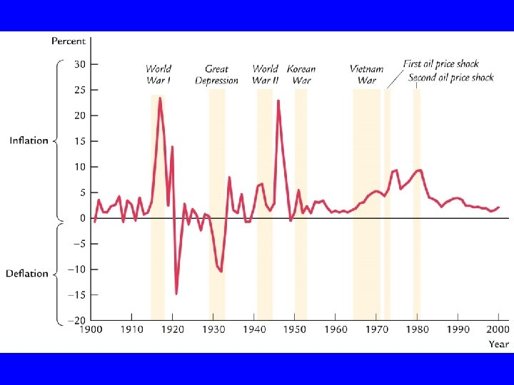
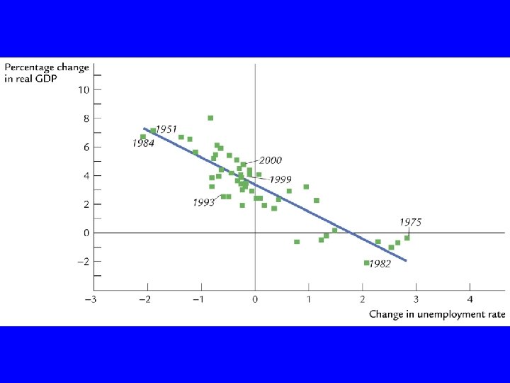
INFLATION AND UNEMPLOYMENT u INFLATION – increases in the price level represent inflation – decreases in the price level represent deflation u EMPLOYMENT – increases in Real GDP reduce unemployment – decreases in Real GDP increase unemployment

SHIFT IN AGGREGATE DEMAND u INCREASE – – AD shifts right price level rises Real GDP rises unemployment falls u DECREASE – – AD shifts left price level falls Real GDP falls unemployment rises

INCREASE IN AD

INCREASE IN AGGREGATE SUPPLY AS curve shifts to the right u price level falls u Real GDP rises u Unemployment falls u

INCREASE IN AS

DECREASE IN AGGREGATE SUPPLY AS shifts to the left u price level rises u Real GDP falls u unemployment rises u

Decrease in AS

Examples Increase in wage rate + Increase in income taxes u Decrease in business taxes + Good weather u Increase in interest rates + Decrease in Foreign national income u Depreciation of US dollar + Increase in oil price u Decrease in expected future income + increase in productivity u

SHORT RUN the short run is defined as a period of time in which at least one input is fixed u for example, firms can change the number of workers relatively easily but it takes longer to build a new plant u plant size is fixed in the short run u

LONG RUN the long run is defined as a period of time long enough to adjust all inputs u firms can make major adjustments in their plant size given enough time u all inputs are variable in the long run u

LONG RUN AGGREGATE SUPPLY the amount of real output u the economy is able to supply u at different price levels u if the economy is at Natural Real GDP u

NATURAL REAL GDP the amount of output u the economy could produce u if it operated at full employment u called Qn or Qf u
 vertical line u at full employment Real GDP u")
LONG RUN AGGREGATE SUPPLY (LRAS) vertical line u at full employment Real GDP u Qn = Qf u
 Curve")
Exhibit 13 Long-Run Aggregate Supply (LRAS) Curve

THREE POSSIBLE STATES OF THE ECONOMY Recessionary gap u Inflationary gap u Full Employment Equilibrium u
")
RECESSIONARY GAP The intersection of SRAS and AD is below (to the left of) the Natural Real GDP (full employment)
 Price Level In this")
Three Possible States of the Economy RECESSIONARY GAP Part (a) Price Level In this diagram, the economy is currently in short-run equilibrium at a Real GDP level of Q 1. QN is Natural Real GDP or the potential output of the economy. Notice that Q 1< QN. When this condition (Q 1< QN) exists, the economy is said to be in a recessionary gap. SRAS 1 1 The economy is here. AD 1 0 Q 1 QN Real GDP
")
INFLATIONARY GAP The intersection of SRAS and AD is above (to the right of) the Natural Real GDP (full employment)
 Price Level SRAS In")
Three Possible States of the Economy INFLATIONARY GAP Part (b) Price Level SRAS In this diagram, the economy is currently in short-run equilibrium at a Real GDP level of Q 1. QN is Natural Real GDP or the potential output of the economy. Notice that Q 1> QN. When this condition (Q 1> QN) exists, the economy is said to be in an inflationary gap. 1 The economy is here. AD 1 0 Q Q 1 Real GDP

FULL EMPLOYMENT EQUILIBRIUM The intersection of SRAS and AD is equal to the Natural Real GDP
 Price Level In this")
Three Possible States of the Economy LONG-RUN EQUILIBRIUM Part (c) Price Level In this diagram, the economy is currently operating at a Real GDP level of Q 1, which happens to be equal to QN. In other words, the economy is producing its Natural Real GDP or potential output. When this condition (Q 1= QN) exists, the economy is said to be in long-run equilibrium. SRAS The economy is here. 1 AD 1 0 QN Q 1 Real GDP
- Slides: 54