macro Topic 9 CHAPTER TEN Aggregate Demand II

macro Topic 9: CHAPTER TEN Aggregate Demand II (chapter 10) macroeconomics fifth edition N. Gregory Mankiw Power. Point® Slides by Ron Cronovich © 2002 Worth Publishers, all rights reserved

Motivation § The Great Depression caused a rethinking of the Classical Theory of the macroeconomy. It could not explain: – Drop in output by 30% from 1929 to 1933 – Rise in unemployment to 25% § In 1936, J. M. Keynes developed a theory to explain this phenomenon. § We will learn a version of this theory, called the ‘IS-LM’ model. CHAPTER 10 Aggregate Demand I 1

Context § Chapter 9 introduced the model of aggregate demand aggregate supply. § Long run – prices flexible – output determined by factors of production & technology – unemployment equals its natural rate § Short run – prices fixed – output determined by aggregate demand – unemployment is negatively related to output CHAPTER 10 Aggregate Demand I 2

Context § This chapter develops the IS-LM model, theory that yields the aggregate demand curve. § We focus on the short run and assume the price level is fixed. CHAPTER 10 Aggregate Demand I 3

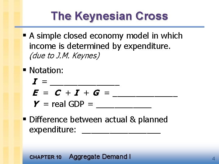
The Keynesian Cross § A simple closed economy model in which income is determined by expenditure. (due to J. M. Keynes) § Notation: I = ________ E = C + I + G = _______ Y = real GDP = ______ § Difference between actual & planned expenditure: _________ CHAPTER 10 Aggregate Demand I 4

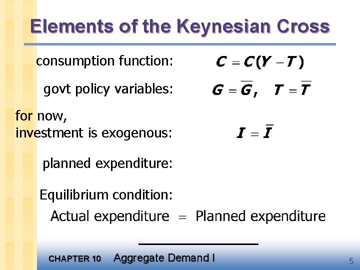
Elements of the Keynesian Cross consumption function: govt policy variables: for now, investment is exogenous: planned expenditure: Equilibrium condition: CHAPTER 10 Aggregate Demand I 5

Graphing planned expenditure E planned expenditure income, output, Y CHAPTER 10 Aggregate Demand I 6

Graphing the equilibrium condition E planned expenditure income, output, Y CHAPTER 10 Aggregate Demand I 7

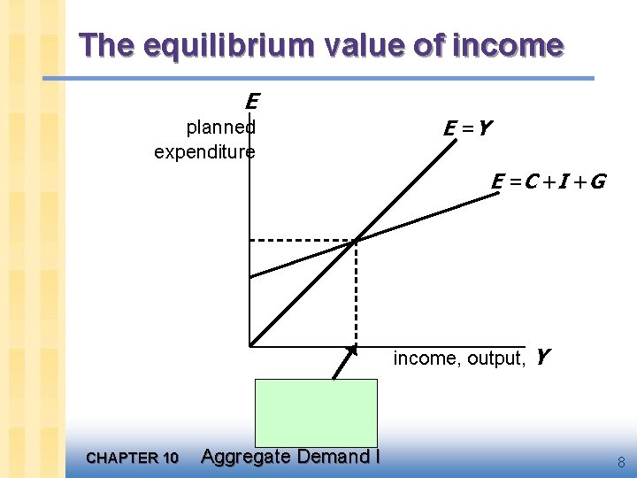
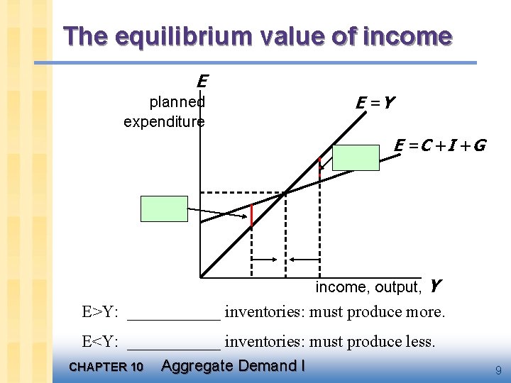
The equilibrium value of income E planned expenditure E =Y E = C +I +G income, output, Y CHAPTER 10 Aggregate Demand I 8

The equilibrium value of income E planned expenditure E =Y E = C +I +G income, output, Y E>Y: ______ inventories: must produce more. E<Y: ______ inventories: must produce less. CHAPTER 10 Aggregate Demand I 9

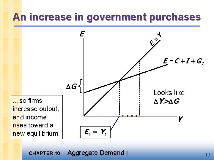
An increase in government purchases = E E Y E = C + I + G 1 G …so firms increase output, and income rises toward a new equilibrium CHAPTER 10 Looks like Y> G Y E 1 = Y 1 Aggregate Demand I 10

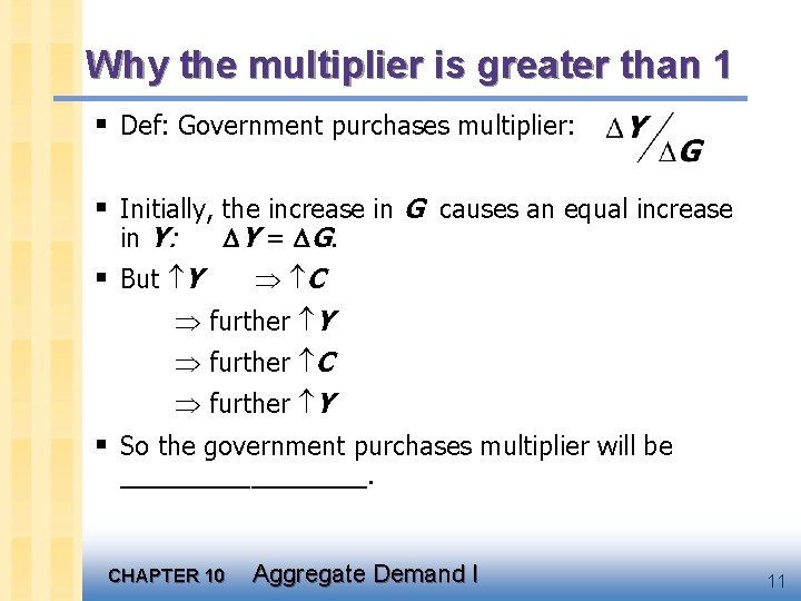
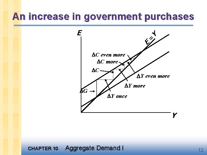
Why the multiplier is greater than 1 § Def: Government purchases multiplier: § Initially, the increase in G causes an equal increase in Y: Y = G. § But Y C further Y further C further Y § So the government purchases multiplier will be _________. CHAPTER 10 Aggregate Demand I 11

An increase in government purchases = E E C even more C G Y Y even more Y more Y once Y CHAPTER 10 Aggregate Demand I 12

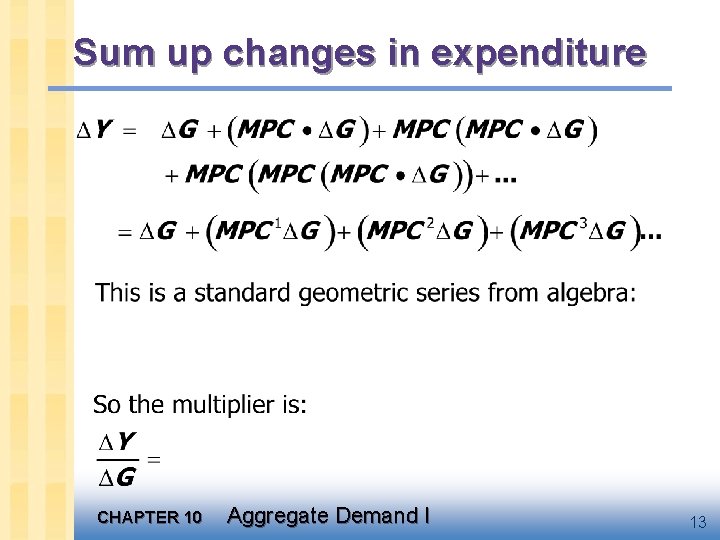
Sum up changes in expenditure CHAPTER 10 Aggregate Demand I 13

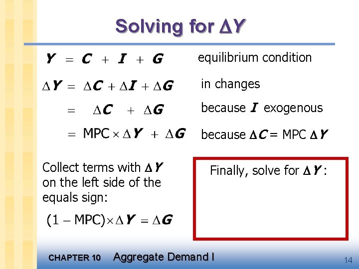
Solving for Y equilibrium condition in changes because I exogenous because C = MPC Y Collect terms with Y on the left side of the equals sign: CHAPTER 10 Finally, solve for Y : Aggregate Demand I 14

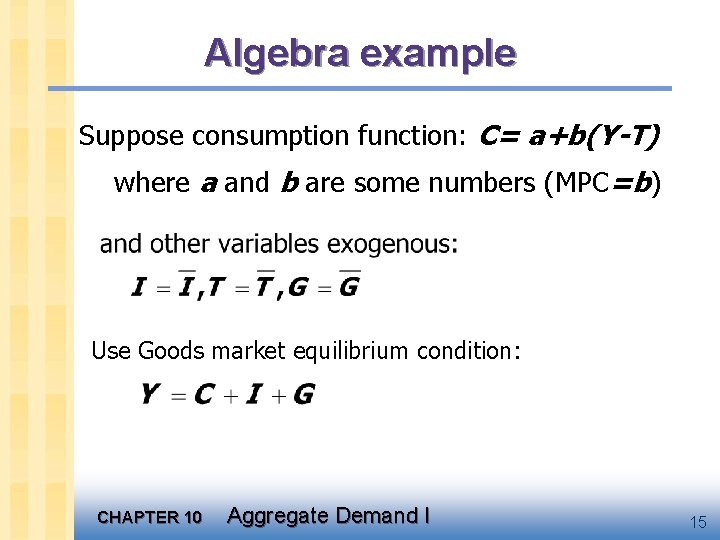
Algebra example Suppose consumption function: C= a+b(Y-T) where a and b are some numbers (MPC=b) Use Goods market equilibrium condition: CHAPTER 10 Aggregate Demand I 15

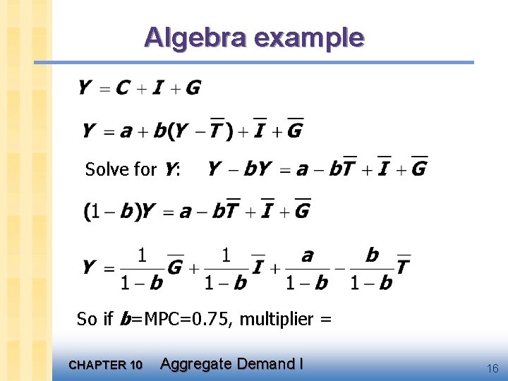
Algebra example Solve for Y: So if b=MPC=0. 75, multiplier = CHAPTER 10 Aggregate Demand I 16

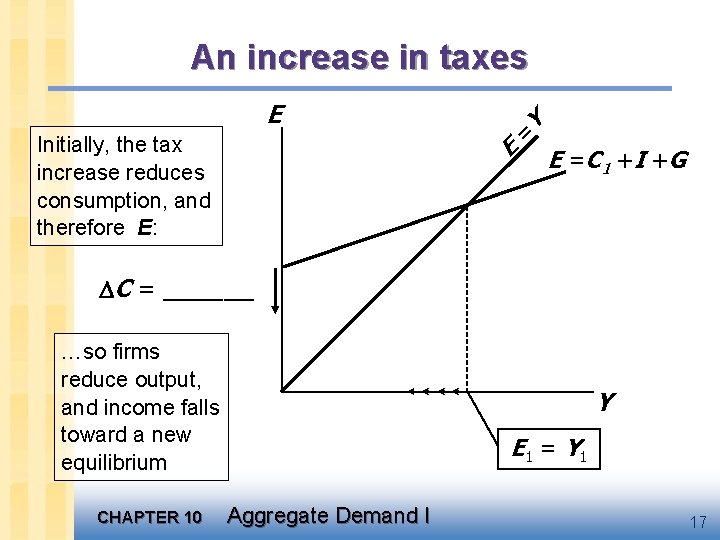
An increase in taxes = E Initially, the tax increase reduces consumption, and therefore E: E Y E = C 1 +I +G C = ______ …so firms reduce output, and income falls toward a new equilibrium CHAPTER 10 Y E 1 = Y 1 Aggregate Demand I 17

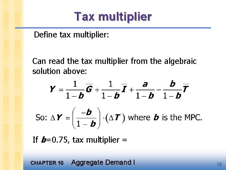
Tax multiplier Define tax multiplier: Can read the tax multiplier from the algebraic solution above: If b=0. 75, tax multiplier = CHAPTER 10 Aggregate Demand I 18

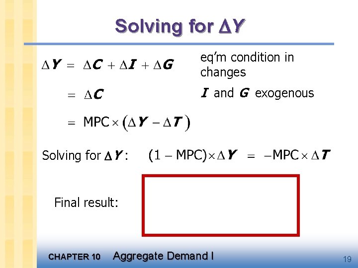
Solving for Y eq’m condition in changes I and G exogenous Solving for Y : Final result: CHAPTER 10 Aggregate Demand I 19

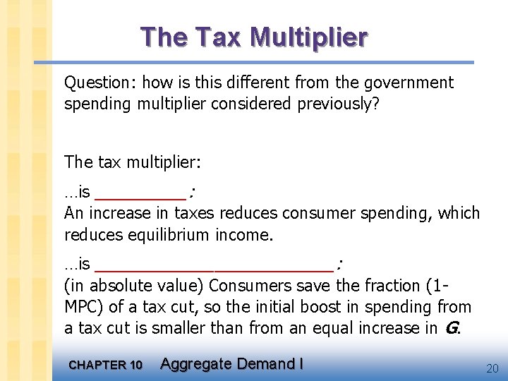
The Tax Multiplier Question: how is this different from the government spending multiplier considered previously? The tax multiplier: …is _____: An increase in taxes reduces consumer spending, which reduces equilibrium income. …is _____________: (in absolute value) Consumers save the fraction (1 MPC) of a tax cut, so the initial boost in spending from a tax cut is smaller than from an equal increase in G. CHAPTER 10 Aggregate Demand I 20

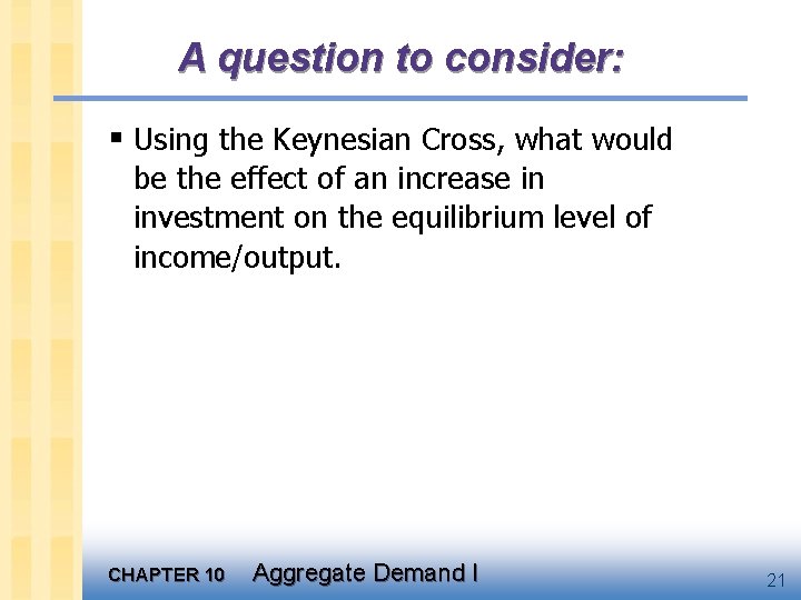
A question to consider: § Using the Keynesian Cross, what would be the effect of an increase in investment on the equilibrium level of income/output. CHAPTER 10 Aggregate Demand I 21

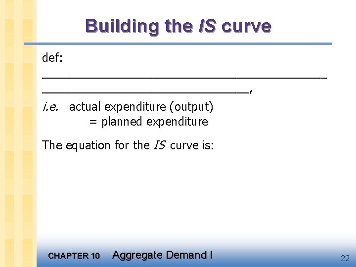
Building the IS curve def: ______________________, i. e. actual expenditure (output) = planned expenditure The equation for the IS curve is: CHAPTER 10 Aggregate Demand I 22

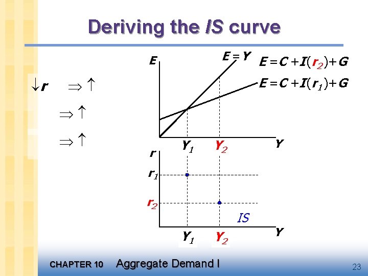
Deriving the IS curve E =Y E =C +I (r )+G 2 E r E =C +I (r 1 )+G r Y 1 Y Y 2 r 1 r 2 IS Y 1 CHAPTER 10 Y 2 Aggregate Demand I Y 23

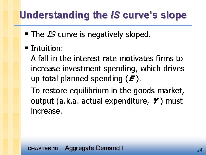
Understanding the IS curve’s slope § The IS curve is negatively sloped. § Intuition: A fall in the interest rate motivates firms to increase investment spending, which drives up total planned spending (E ). To restore equilibrium in the goods market, output (a. k. a. actual expenditure, Y ) must increase. CHAPTER 10 Aggregate Demand I 24

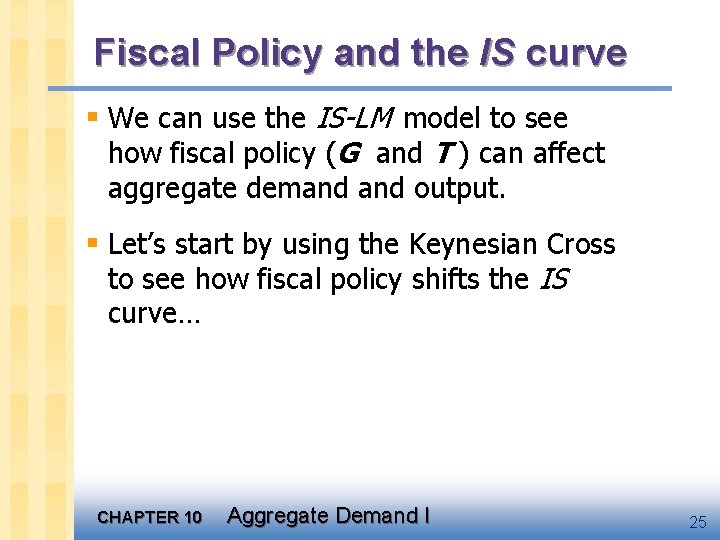
Fiscal Policy and the IS curve § We can use the IS-LM model to see how fiscal policy (G and T ) can affect aggregate demand output. § Let’s start by using the Keynesian Cross to see how fiscal policy shifts the IS curve… CHAPTER 10 Aggregate Demand I 25

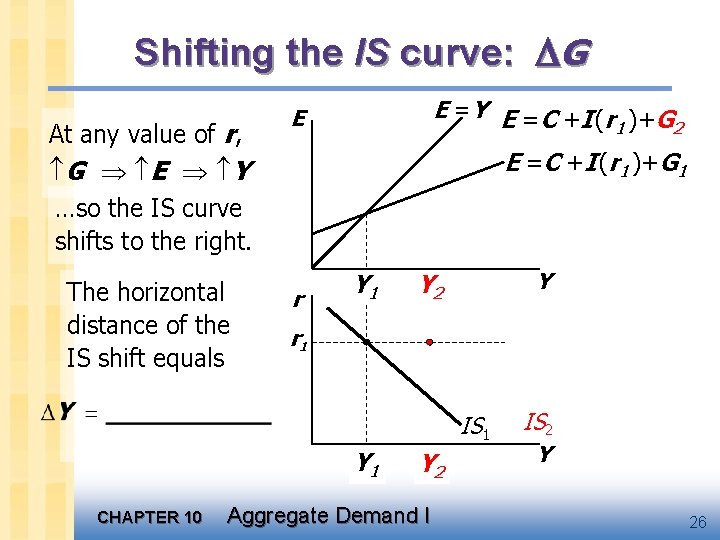
Shifting the IS curve: G At any value of r, G E Y …so the IS curve shifts to the right. The horizontal distance of the IS shift equals E =Y E =C +I (r )+G 1 2 E E =C +I (r 1 )+G 1 r Y 1 Y Y 2 r 1 IS 1 Y 1 CHAPTER 10 Y 2 Aggregate Demand I IS 2 Y 26

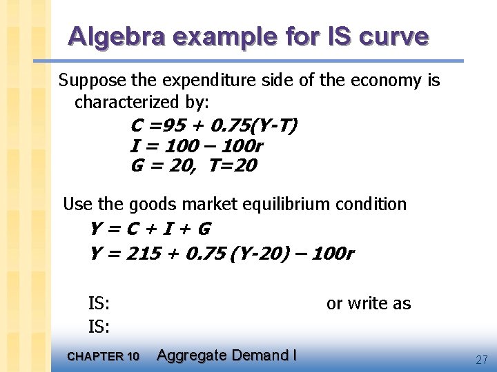
Algebra example for IS curve Suppose the expenditure side of the economy is characterized by: C =95 + 0. 75(Y-T) I = 100 – 100 r G = 20, T=20 Use the goods market equilibrium condition Y=C+I+G Y = 215 + 0. 75 (Y-20) – 100 r IS: CHAPTER 10 or write as Aggregate Demand I 27

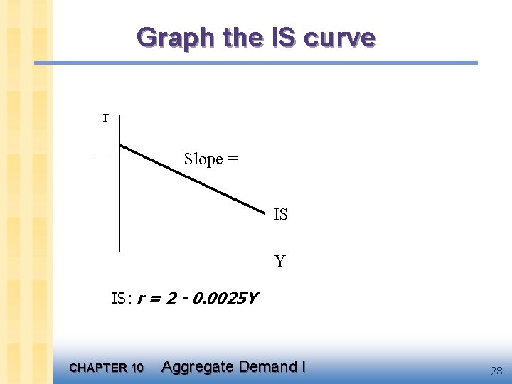
Graph the IS curve r __ Slope = IS Y IS: r = 2 - 0. 0025 Y CHAPTER 10 Aggregate Demand I 28

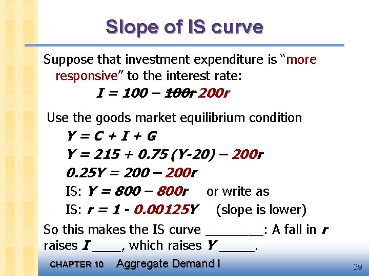
Slope of IS curve Suppose that investment expenditure is “more responsive” to the interest rate: I = 100 – 100 r 200 r Use the goods market equilibrium condition Y=C+I+G Y = 215 + 0. 75 (Y-20) – 200 r 0. 25 Y = 200 – 200 r IS: Y = 800 – 800 r or write as IS: r = 1 - 0. 00125 Y (slope is lower) So this makes the IS curve ____: A fall in r raises I ____, which raises Y _____. CHAPTER 10 Aggregate Demand I 29

Building the LM Curve: Theory of Liquidity Preference § due to John Maynard Keynes. § A simple theory in which the interest rate is determined by money supply and money demand. CHAPTER 10 Aggregate Demand I 30

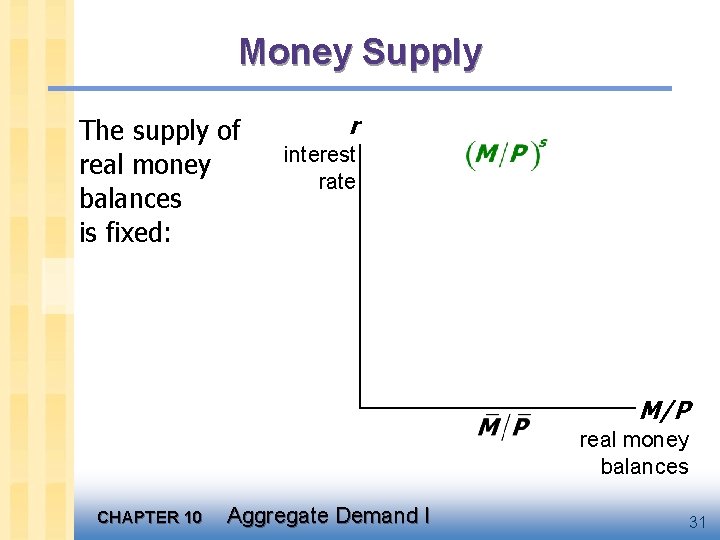
Money Supply The supply of real money balances is fixed: r interest rate M/P real money balances CHAPTER 10 Aggregate Demand I 31

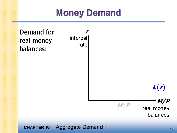
Money Demand for real money balances: r interest rate L (r ) M/P real money balances CHAPTER 10 Aggregate Demand I 32

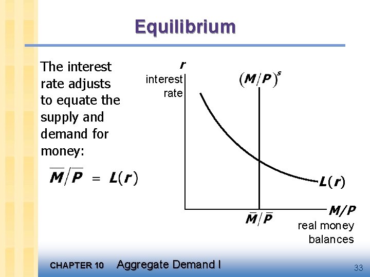
Equilibrium The interest rate adjusts to equate the supply and demand for money: r interest rate L (r ) M/P real money balances CHAPTER 10 Aggregate Demand I 33

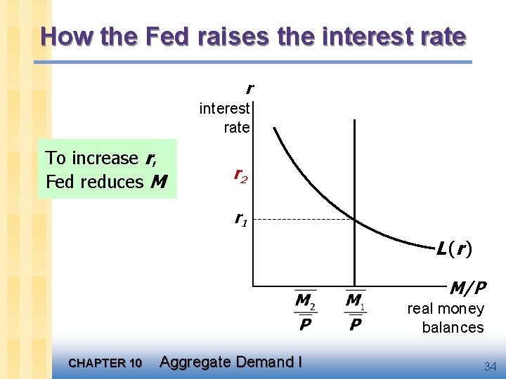
How the Fed raises the interest rate r interest rate To increase r, Fed reduces M r 2 r 1 L (r ) M/P real money balances CHAPTER 10 Aggregate Demand I 34

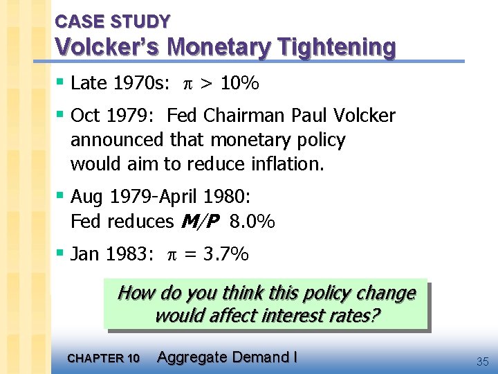
CASE STUDY Volcker’s Monetary Tightening § Late 1970 s: > 10% § Oct 1979: Fed Chairman Paul Volcker announced that monetary policy would aim to reduce inflation. § Aug 1979 -April 1980: Fed reduces M/P 8. 0% § Jan 1983: = 3. 7% How do you think this policy change would affect interest rates? CHAPTER 10 Aggregate Demand I 35

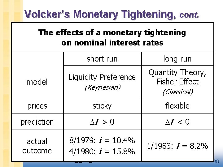
Volcker’s Monetary Tightening, cont. The effects of a monetary tightening on nominal interest rates model short run long run Liquidity Preference Quantity Theory, Fisher Effect (Keynesian) (Classical) prices sticky flexible prediction i > 0 i < 0 actual outcome 8/1979: i = 10. 4% 4/1980: i = 15. 8% 1/1983: i = 8. 2% CHAPTER 10 Aggregate Demand I 36

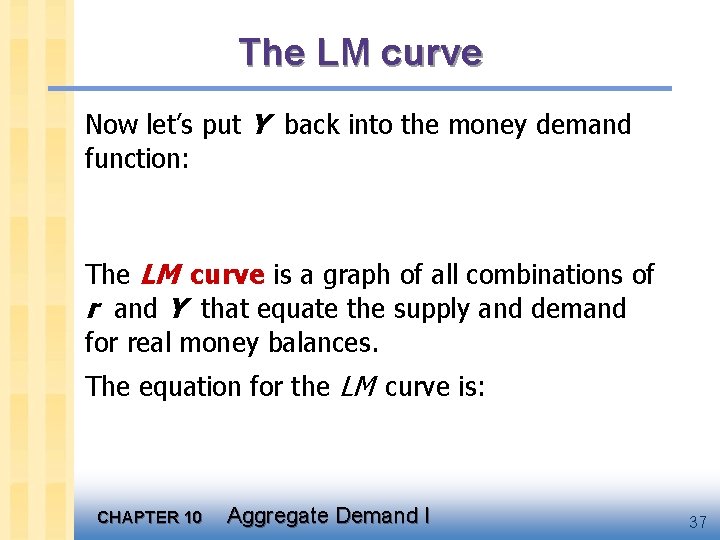
The LM curve Now let’s put Y back into the money demand function: The LM curve is a graph of all combinations of r and Y that equate the supply and demand for real money balances. The equation for the LM curve is: CHAPTER 10 Aggregate Demand I 37

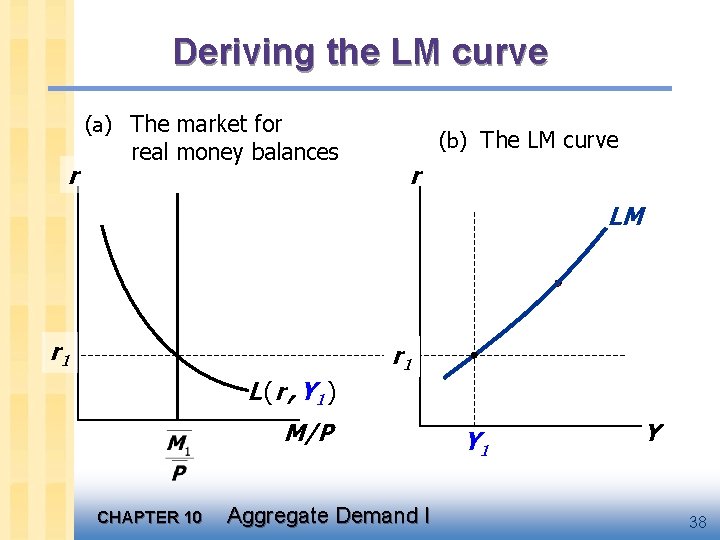
Deriving the LM curve (a) The market for r real money balances (b) The LM curve r LM r 1 L ( r , Y 1 ) M/P CHAPTER 10 Aggregate Demand I Y 1 Y 38

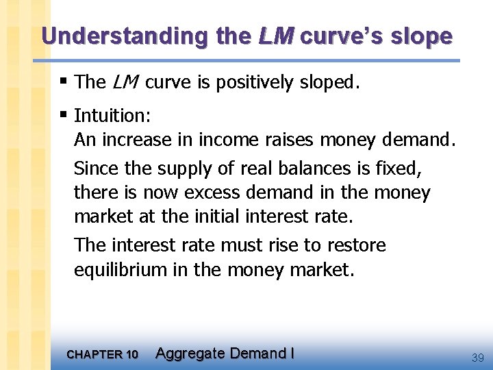
Understanding the LM curve’s slope § The LM curve is positively sloped. § Intuition: An increase in income raises money demand. Since the supply of real balances is fixed, there is now excess demand in the money market at the initial interest rate. The interest rate must rise to restore equilibrium in the money market. CHAPTER 10 Aggregate Demand I 39

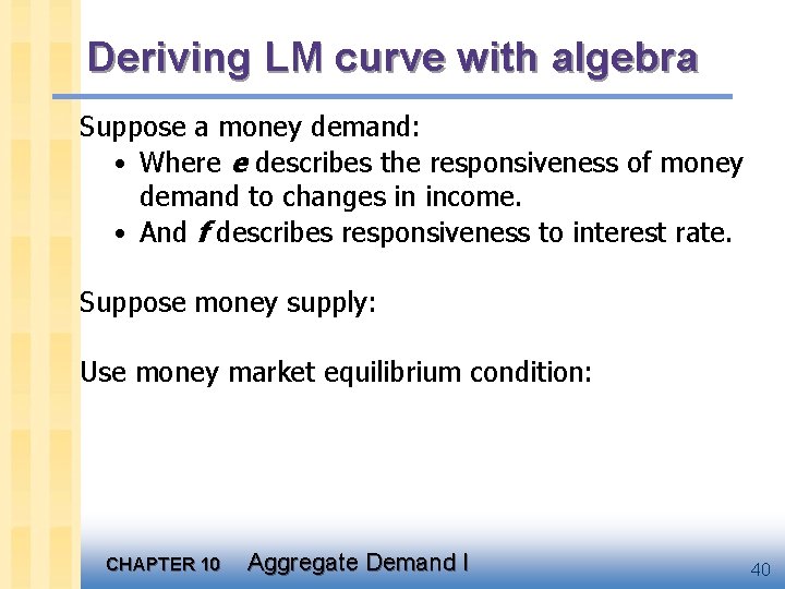
Deriving LM curve with algebra Suppose a money demand: • Where e describes the responsiveness of money demand to changes in income. • And f describes responsiveness to interest rate. Suppose money supply: Use money market equilibrium condition: CHAPTER 10 Aggregate Demand I 40

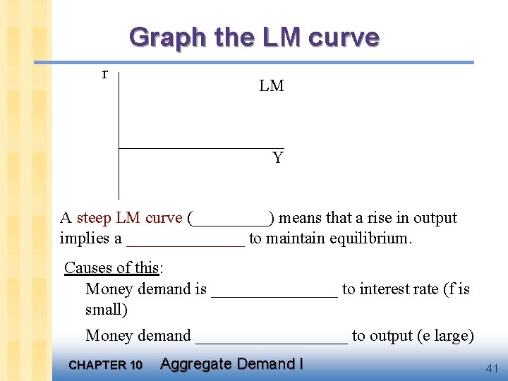
Graph the LM curve r LM Y A steep LM curve (_____) means that a rise in output implies a _______ to maintain equilibrium. Causes of this: Money demand is ________ to interest rate (f is small) Money demand _________ to output (e large) CHAPTER 10 Aggregate Demand I 41

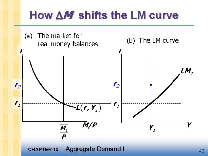
How M shifts the LM curve (a) The market for r real money balances (b) The LM curve r LM 1 r 2 r 1 L ( r , Y 1 ) M/P CHAPTER 10 Aggregate Demand I Y 1 Y 42

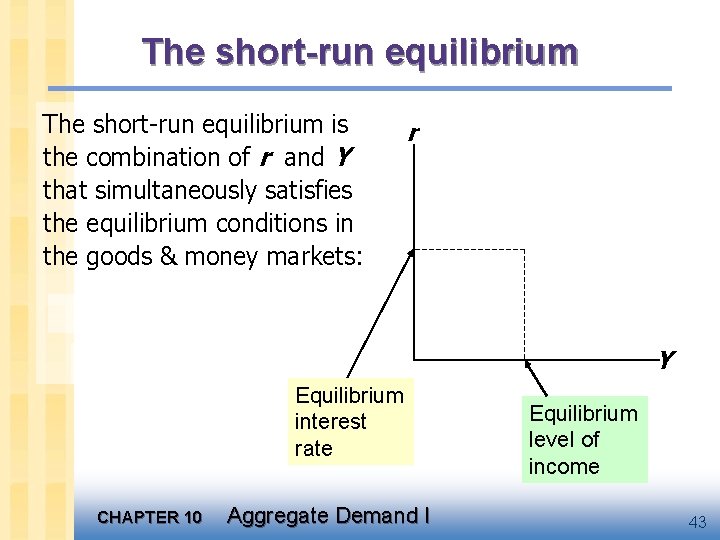
The short-run equilibrium is the combination of r and Y that simultaneously satisfies the equilibrium conditions in the goods & money markets: r Y Equilibrium interest rate CHAPTER 10 Aggregate Demand I Equilibrium level of income 43

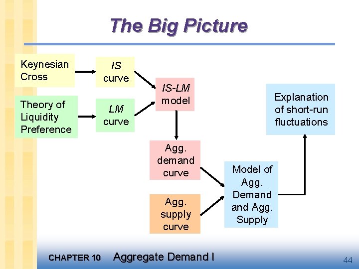
The Big Picture Keynesian Cross Theory of Liquidity Preference IS curve LM curve IS-LM model Agg. demand curve Agg. supply curve CHAPTER 10 Aggregate Demand I Explanation of short-run fluctuations Model of Agg. Demand Agg. Supply 44

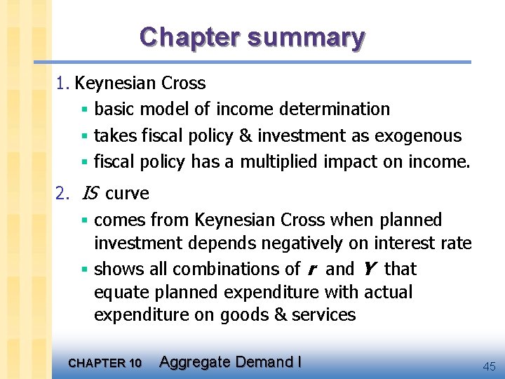
Chapter summary 1. Keynesian Cross § basic model of income determination § takes fiscal policy & investment as exogenous § fiscal policy has a multiplied impact on income. 2. IS curve § comes from Keynesian Cross when planned investment depends negatively on interest rate § shows all combinations of r and Y that equate planned expenditure with actual expenditure on goods & services CHAPTER 10 Aggregate Demand I 45

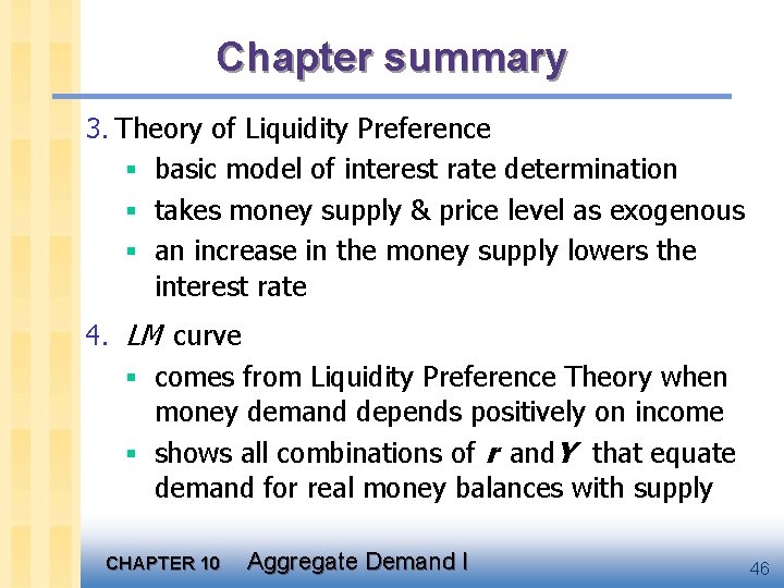
Chapter summary 3. Theory of Liquidity Preference § basic model of interest rate determination § takes money supply & price level as exogenous § an increase in the money supply lowers the interest rate 4. LM curve § comes from Liquidity Preference Theory when money demand depends positively on income § shows all combinations of r and. Y that equate demand for real money balances with supply CHAPTER 10 Aggregate Demand I 46

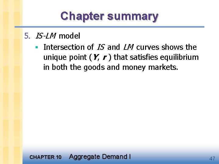
Chapter summary 5. IS-LM model § Intersection of IS and LM curves shows the unique point (Y, r ) that satisfies equilibrium in both the goods and money markets. CHAPTER 10 Aggregate Demand I 47