Macro Theory The ASAD Model Part 1 The

Macro Theory: The AS/AD Model Part 1 – The Basics Part 2 – The Keynesian View Dr. D. Foster – ECO 285 – Macroeconomics

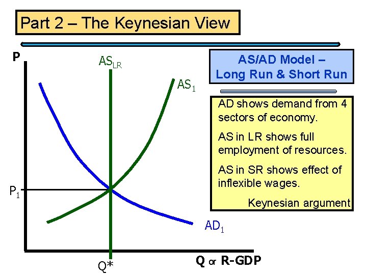
Part 2 – The Keynesian View P ASLR AS 1 AS/AD Model – Long Run & Short Run AD shows demand from 4 sectors of economy. AS in LR shows full employment of resources. AS in SR shows effect of inflexible wages. P 1 Keynesian argument AD 1 Q* Q or R-GDP

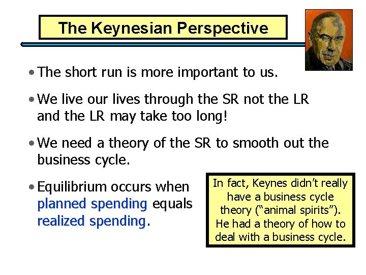
The Keynesian Perspective • The short run is more important to us. • We live our lives through the SR not the LR and the LR may take too long! • We need a theory of the SR to smooth out the business cycle. • Equilibrium occurs when planned spending equals realized spending In fact, Keynes didn’t really have a business cycle theory (“animal spirits”). He had a theory of how to deal with a business cycle.

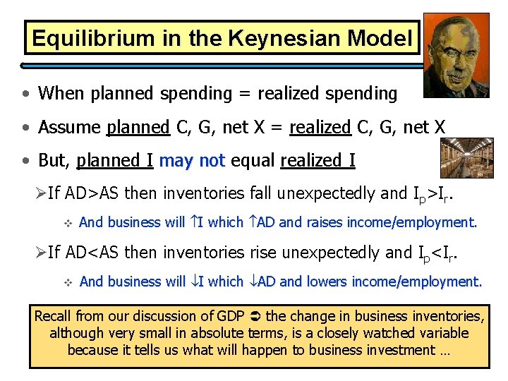
Equilibrium in the Keynesian Model • When planned spending = realized spending • Assume planned C, G, net X = realized C, G, net X • But, planned I may not equal realized I ØIf AD>AS then inventories fall unexpectedly and Ip>Ir. v And business will I which AD and raises income/employment. ØIf AD<AS then inventories rise unexpectedly and Ip<Ir. v And business will I which AD and lowers income/employment. Recall from our discussion of GDP the change in business inventories, although very small in absolute terms, is a closely watched variable because it tells us what will happen to business investment …

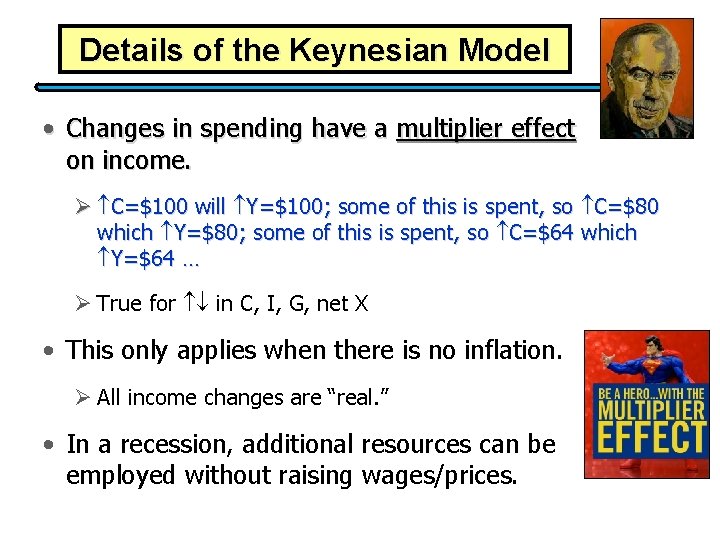
Details of the Keynesian Model • Changes in spending have a multiplier effect on income. Ø C=$100 will Y=$100; some of this is spent, so C=$80 which Y=$80; some of this is spent, so C=$64 which Y=$64 … Ø True for in C, I, G, net X • This only applies when there is no inflation. Ø All income changes are “real. ” • In a recession, additional resources can be employed without raising wages/prices.

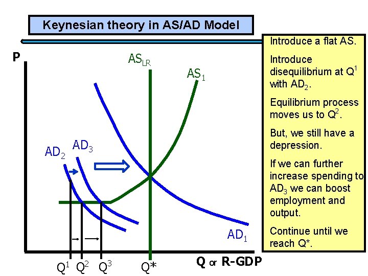
Keynesian theory in AS/AD Model Introduce a flat AS. P ASLR Introduce disequilibrium at Q 1 with AD 2. AS 1 Equilibrium process moves us to Q 2. AD 2 But, we still have a depression. AD 3 If we can further increase spending to AD 3 we can boost employment and output. AD 1 Q 2 Q 3 Q* Q or R-GDP Continue until we reach Q*.

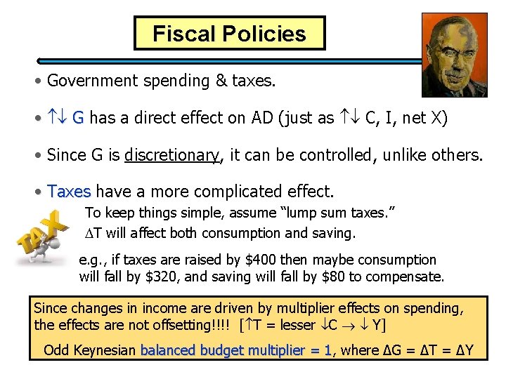
Fiscal Policies • Government spending & taxes. • G has a direct effect on AD (just as C, I, net X) • Since G is discretionary, it can be controlled, unlike others. • Taxes have a more complicated effect. To keep things simple, assume “lump sum taxes. ” T will affect both consumption and saving. e. g. , if taxes are raised by $400 then maybe consumption will fall by $320, and saving will fall by $80 to compensate. Since changes in income are driven by multiplier effects on spending, the effects are not offsetting!!!! [ T = lesser C Y] Odd Keynesian balanced budget multiplier = 1, 1 where ∆G = ∆T = ∆Y

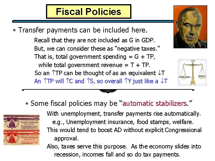
Fiscal Policies • Transfer payments can be included here. Recall that they are not included as G in GDP. But, we can consider these as “negative taxes. ” That is, total government spending = G + TP, while total government revenue = T + TP. So an TP can be thought of as an equivalent T An TP will C and S, so overall Y just like a T • Some fiscal policies may be “automatic stabilizers. ” stabilizers With unemployment, transfer payments rise automatically. e. g. , Unemployment insurance, food stamps, welfare. This would tend to boost AD without explicit Congressional approval. Also, taxes serve this purpose. As the economy slides into recession, incomes fall and so do tax payments.

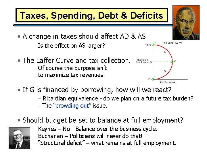
Taxes, Spending, Debt & Deficits • A change in taxes should affect AD & AS Is the effect on AS larger? • The Laffer Curve and tax collection. Of course the purpose isn’t to maximize tax revenues! • If G is financed by borrowing, how will we react? - Ricardian equivalence - do we plan on a future tax burden? - The “crowding out” out issue. • Should budget be set to balance at full employment? Keynes – No! Balance over the business cycle. Buchanan – Politicians will never do that! “Structural deficit” – what remains at full employment.

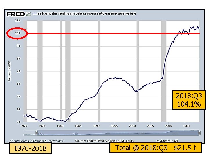
2018: Q 3 104. 1% 1970 -2018 Total @ 2018: Q 3 $21. 5 t

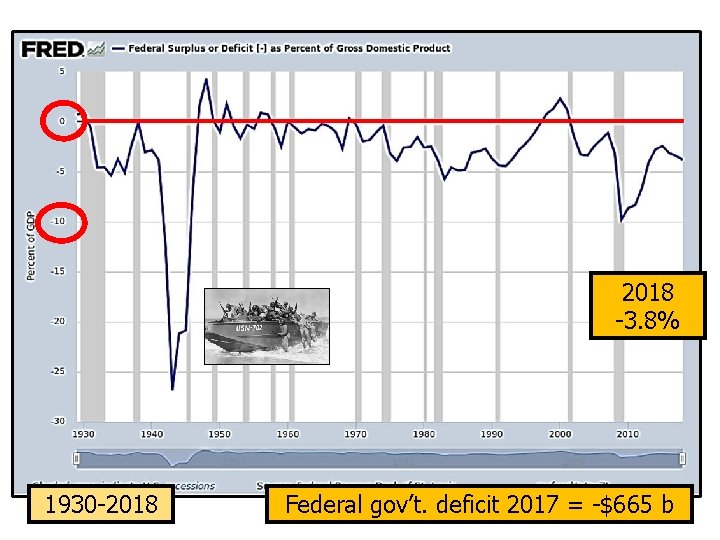
2018 -3. 8% 1930 -2018 Federal gov’t. deficit 2017 = -$665 b

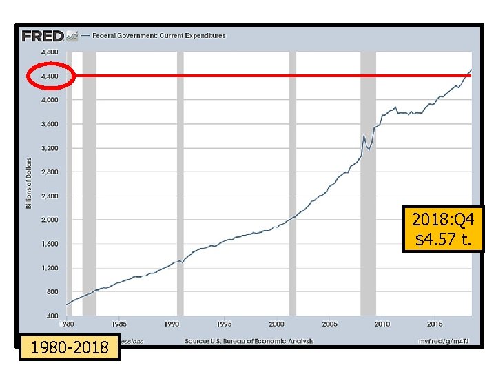
2018: Q 4 $4. 57 t. 1980 -2018

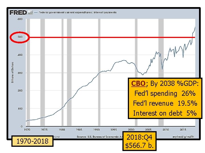
CBO; By 2038 %GDP: Fed’l spending 26% Fed’l revenue 19. 5% Interest on debt 5% 1970 -2018: Q 4 $566. 7 b.

Macro Theory: The AS/AD Model Part 1 – The Basics Part 2 – The Keynesian View Dr. D. Foster – ECO 285 – Macroeconomics