Macro Review Day 2 The Spending Multiplier multiplier

Macro Review Day #2

The Spending Multiplier • multiplier effect: increase in GDP greater (or less) than the increase (or decrease) in spending *a spending increase of $1 creates more than $1 of GDP • Spending Multiplier = 1/MPS OR 1/1 -MPC Ex: Consumers spend 0. 8 & save 0. 2 of extra income. Multiplier? 1/. 2 = 5

The Tax Multiplier • When gov’t taxes…multiplier works in reverse (money is leaving the circular flow) o TAX CUT = higher multiplier

The Balanced Budget Multiplier • Gov’t spending = Gov’t revenues (taxes) • BBM always = 1 • MPC/ MPS = 1

Aggregate Demand (AD) & Aggregate Supply (AS)

Aggregate Demand Curve Price level A reduction in the price level will increase the quantity of goods & services demanded P 1 P 2 AD Y 1 Y 2 Downward Sloping Demand Curve: total GDPR from private, public & foreign sector Goods & Services (real GDP)

Causes of movements on AD curve: Wealth Effect: at higher PL the real value (or purchasing power) of wealth diminishes Interest-Rate Effect: as PL rise so will i% - higher PL’s increase the demand for money…i%? Foreign Purchases Effect: domestic PL rises, U. S. buyers purchase more imports…dollar appreciated or depreciated?

Shifts in Aggregate Demand (non-price level determinants) I. Change in Consumer Spending: - wealth, expectations, debt, taxes II. Change in Investment Spending: - interest rates, profits, business taxes, tech. , inventory levels III. Change in Government Spending IV. Change in Net Exports -national income abroad & exchange rates

Price Shifts in Aggregate Demand level AD 1 AD 0 AD 2 Goods & Services (real GDP) • Increase in real wealth increases aggregate demand, shifting entire curve to right (AD 0 to AD 1) • Reduction in real wealth decreases demand for goods & services, causing AD to shift to left (AD 0 to AD 2)

1. Explain how and why each of the following factors would influence current aggregate demand in the United States: (a) An increased fear of a recession. (b) An increased fear of inflation. (c) The rapid growth of real income in Canada & W. Europe. (d) A reduction in the real interest rate. (e) A higher price level.

Short-Run (SRAS) & Long-Run (LRAS) Aggregate Supply Short-run AS: input prices are “sticky” & do NOT adjust to PL o In SR GDPR directly related to PL o Long-run AS: input prices completely flexible & households/businesses adjust to changes in PL o In LR GDPR independent of PL! o

SRAS Curve Price level SRAS (P 100) An increase in the price level will increase the quantity supplied in the short run. P 105 P 100 P 95 Y 1 Upward sloping supply curve Y 2 Y 3 Goods & Services (real GDP)

LRAS Curve Price level LRAS Change in price level does not affect quantity supplied in the long run. YF (full employment rate of output) Goods & Services (real GDP) -full employment rate of output (YF): maximum sustainable output - LRAS curve is always vertical!

Shifts in Aggregate Supply (non-price level determinants) Factors that change SRAS: I. Change in Resource Prices II. Change in Productivity: -training & tech. III. Change in Legal-Institutional Environment: -business taxes, subsidies, gov’t regs

Shifts in Aggregate Supply Price level LRAS 1 YF, 1 Price level LRAS 2 YF, 2 SRAS 1 SRAS 2 Goods & Services (real GDP) • Increases in resources & tech. , or government deregulation EXPAND potential output (shift LRAS to right)

1. Indicate how each of the following would influence U. S. aggregate supply in the short run: (a) An increase in real wage rates. (b) A severe freeze that destroys half the orange crop in Florida. (c) An increase in the expected rate of inflation in the future. (d) An increase in the world price of oil. (e) Abundant rainfall during the growing season of agricultural states.

Short-Run Equilibrium Price level SRAS(P 100) Intersection of AD and SRAS determines output P AD Y Goods & Services (real GDP)

Long-Run Equilibrium Price level LRAS SRAS(P 100) Quantity demanded just equals quantity supplied P 100 YF AD 100 Goods & Services (full employment rate of output) (real GDP) • current output (YF) = potential GDP (full employment)

SR Increase in AD Price level LRAS SRAS 1 Short-run effects of an unanticipated increase in AD P 105 P 100 AD 2 YF Y 2 • Effect of SR increase in AD? ? ? demand-pull inflation AD 1 Goods & Services (real GDP)

SR Decrease in AD Price level LRAS SRAS 1 Short-run effects of an unanticipated reduction in AD P 100 P 95 Y 2 YF AD 2 AD 1 Goods & Services (real GDP) • Effects of SR decrease in AD? ? ? - recessionary output & cyclical unemployment

The “Sticky” Short-Run vs. “Flexible” Long-Run Ratchet Effect: PL’s "sticky" or inflexible in downward direction Reasons: wage contracts, morale & productivity, minimum wage, “menu” costs, price wars

LRAS Shift Outward Price level LRAS 1 LRAS 2 SRAS 1 SRAS 2 P 1 P 2 AD YFF 1 YF 2 Goods & Services (real GDP) • LRAS shift outward = economic growth • Shift inward of SRAS? – PL increases & cost-push inflation

Aggregate Consumption Schedule Planned Consumption Expenditures 12 45º Line (trillions of dollars) Saving C 9 6 Dis-saving 3 45º 3 6 9 12 Real Disposable Income (trillions of dollars) Keynesian model: positive relationship b/n consumption & income

Free Response Clues: -Do NOT restate question! -Use correct economic jargon! -Use outline #’s will answering question! -You CAN use short-hand (AD ↑, PL ↓). -Analyzing a problem!!! -“Show” means graph, “Indicate” means direction (↑ or ↓), and “Explain” means explain!

1. Assume that the United States economy is currently in equilibrium at the fullemployment level of real gross domestic product. (a) Draw a correctly labeled graph of aggregate demand aggregate supply showing each of the following in the United States. (i) Output level (ii) Price level (b) Japan is a major importer of United States products. Assume that the Japanese economy goes into a recession. (i) Explain the impact of the Japanese recession on the United States equilibrium output and price levels. (ii) Show the effects on your graph in part (a). (c) Assume that the Federal Reserve takes action to curb the effects of the Japanese recession on the United States economy. (i) What open-market operations would the Federal Reserve undertake? (ii) Use a correctly labeled graph of the money market to show the Federal Reserve policy action will affect the nominal interest rate. (iii) Explain how the change in the nominal interest rate in part (c) (ii) will affect aggregate demand, price level, and real output in the United States. (d) Define the real interest rate. (e) Indicate the effect of the open-market operation you identified in part (C) (i) on the real interest rate in the United States.

Productivity = total output/total inputs • More productivity = lower costs • SRAS?

PPC Growth Capital Goods . . PPC Consumer Goods PPC 1

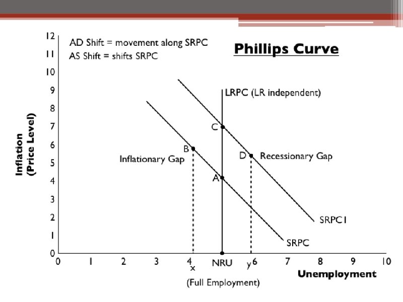
SR PHILLIPS CURVE 7 SR tradeoff: inflation declines, unemployment increases 6 5 Inflation 4 3 2 1 0 1 2 3 4 5 Unemployment 6 7

LR Phillips Curve Inflation LRPC Unemployment *Natural rate of unemployment constant

Fiscal Policy • Gov’t efforts to promote FE output & price stability • Recession = expansionary policy o increase G o decrease T • Inflation = contractionary policy o decrease G o increase T WHICH IS MORE OF A DIRECT INJECTION? ? ?

Expansionary Fiscal Policy SRAS LRAS PL P 1 P ↑ AD 2 AD 1 Y YF GDPR IN RECESSION: ↑G, AD↑, GDPR↑, PL↑, u%↓, π%↑ OR T↓, DI↑, C↑, AD↑, GDPR↑, PL↑, u%↓, π%↑

Discretionary v. Automatic Fiscal Policies • Discretionary: increase or decrease G &T Problems: • time lags • political motivations • Automatic: unemployment benefits, marginal tax rates

Expansionary fiscal policy side-effect: ‘Crowding-out’ SLF i% i% r 1 r DLF 1 ID DLF q q 1 QLF I 1 I Gov’t deficit spending (G↑ or T↓) causes DLF↑, i%↑, IG↓ IG

Decline in Private Investment Increase In Budget Deficit Higher Real Interest Rates Inflow of Financial Capital from Abroad Appreciation of the Dollar Crowding-Out in an Open Economy Decline in Net Exports

‘Crowding-In’ Contractionary Fiscal Policy Side-effect: – ‘crowding-in’ of IG & XN

Money: o o o medium of exchange store of value unit of account Supply of Money: • Federal Reserve controls SM o M 1 (currency, coin, demand deposits) o M 2 (M 1, time deposits, mutual funds)

Federal Reserve Districts Kansas City Minneapolis Chicago 9 1 Cleveland 2 7 3 12 San Francisco 4 Boston New York Philadelphia Washington, D. C. (Board of Governors) 10 8 5 Richmond Atlanta 6 11 St. Louis Dallas There are 12 Federal Reserve districts. Each district bank monitors the commercial banks in their region and assists them with the clearing of checks. The Board of Governors of the Fed is in Washington D. C.

“Velocity” of Money: MV = PQ M = money supply V = velocity of spending P = price level (PL on the AS/AD diagram) Q = GDPR PQ = Nominal GDP

The Money Market • market where Fed & users of money interact • nominal interest rates (i%) • money demand (MD): households, firms, gov’t & foreign sector • money supply (MS): Fed determined *↓i% = ↑bond prices; ↑i% = ↓bond prices

The Money Market i% MS i MD Q QM -MD downward sloping: i% is opportunity cost of holding money - MS vertical: independent of i%

i% Increase in MD MS i 2 ↑ i 1 MD 2 MD 1 Q QM • MD dependent on PL & GDPR • Nominal GDP↑: MD↑: i%↑

i% Increase in MS MS 1 MS 2 ↑ i 1 i 2 MD Q 1 Q 2 QM Expansionary Monetary Policy: MS↑: i%↓ Contractionary Monetary Policy: MS↓: i%↑

Reserve Requirement • Fed requirement for banks to have cash reserves • Required Reserve Ratio • % of demand deposits (checking account balances) • typically RR% = 10% • Excess reserves are loaned out excess reserves = actual reserves - required reserves

Money Multiplier • shows impact of a change in demand deposits on MS Money multiplier = 1/ reserve ratio o Ex. : Reserve ratio is 25%, money multiplier? o 1/. 25 = 4 Maximum money creation = excess reserves x M multiplier • actual deposit multiplier less than potential: • Some will hold currency • Some banks may not use all excess reserves

Monetary Policy • Efforts by central banks (ie: The Fed) to promote full employment, PL stability, & LR growth • control of MS (i%) Expansionary (Easy Money): • fight a recession Contractionary (Tight Money): • counteract inflation TOOLS: • Required Reserve Ratio • Discount Rate • Open Market Operations (OMO) • Term Auction Facility (TAF)…NEW!

TOOLS OF THE FED 1. RR%: • RR%↓ = MS↑ (easy money) • RR%↑ = MS↓ (tight money) 2. Discount rate (“window”): i% banks pay the Fed for overnight loans to meet RR% • Discount Rate%↓ = MS↑ (easy money) • Discount Rate%↑ = MS↓ (tight money) 3. OMO: purchase & sale of gov’t securities by Fed o o Fed buys bonds = MS↑ = easy $ Fed sells bonds = MS ↓ = tight $ 4. TAF: started in 2007 to promote discount window

i% MS MS 1 Graphing Expansionary Monetary Policy i% Fed buys bonds, ↑TAF loans, or ↓discount rate i i i 1 MD Q Q 1 QM ID I I 1 IG LRAS PL SRAS P 1 P AD Y YF AD 1 GDPR

1. Assume that the United States economy is currently in equilibrium at the fullemployment level of real gross domestic product. (a) Draw a correctly labeled graph of aggregate demand aggregate supply showing each of the following in the United States. (i) Output level (ii) Price level (b) Japan is a major importer of United States products. Assume that the Japanese economy goes into a recession. (i) Explain the impact of the Japanese recession on the United States equilibrium output and price levels. (ii) Show the effects on your graph in part (a). (c) Assume that the Federal Reserve takes action to curb the effects of the Japanese recession on the United States economy. (i) What open-market operations would the Federal Reserve undertake? (ii) Use a correctly labeled graph of the money market to show the Federal Reserve policy action will affect the nominal interest rate. (iii) Explain how the change in the nominal interest rate in part (c) (ii) will affect aggregate demand, price level, and real output in the United States. (d) Define the real interest rate. (e) Indicate the effect of the open-market operation you identified in part (C) (i) on the real interest rate in the United States.

• trade deficit: “unfavorable balance of trade, ” or imports exceeding exports • trade surplus: “favorable balance of trade, ” or exports exceed imports

Export Supply: • At the world price of Pw, the quantity (Qp – Qc) is exported Price U. S. Market Price World Market S w S d Pw a Pn b Sw Pw c Dw Dd Qc U. S. exports Qn Q p Soybeans (bushels) Qw Soybeans (bushels)

Import Demand: • At price Pw, U. S. consumers import (Qc – Qp) Price U. S. Market Price World Market S S d a Pn Pw w b c Sw Pw Dd Q p Qn U. S. imports Qc Soybeans (bushels) Dw Qw Soybeans (bushels)

Effects of Trade Protection trade protection: gov’t policies that limit imports - tariffs & import quotas - both produce “deadweight losses” tariff: tax on imports (raises domestic price) import quota: legal limit on Q of imports

Impacts of Tariff

Balance of Payments • Money flows b/n U. S. & World o o inflows = CREDITS outflows = DEBITS • Balance of Payments: o o Current Account (XN; net foreign income; net transfers) Capital/Financial Account (FDI) o o o Toyota Factory in TX = CREDIT Intel Factory Costa Rica = DEBIT Official Reserves Account (Fed foreign currency)

What causes Capital/Financial Flows? • differences in rates of return • Ceteris Paribus: $ flows toward higher returns r% SLF 1 SLF China SLF USA r% SLF 1 DLF USA DLF China Debit to the Chinese Capital Account QLF China Credit to the U. S. Capital Account QLF USA

Foreign Exchange (FOREX) • buying & selling of currency • Fixed Exchange Rate: pegged to a set value • exchange rates determined in FOREX markets o o o price of a currency ↑ supply = depreciation ↓ supply = appreciation ↑ demand = appreciation ↓ demand = depreciation Ex. If German tourists flock to America to go shopping?

Exports & Imports • Appreciation = relatively cheaper foreign goods • imports ↑ • Depreciation = relatively cheaper domestic goods • exports ↑

Exchange Rate Determinants • • Consumer Tastes Relative Income Relative Price Level Speculation Ex: If the price level is higher in Canada than in the United States? Ex: If U. S. investors expect that Swiss interest rates will climb in the future?

$/£ Increase in Demand for £ relative to $ S£ e 1 e D£ q q 1 D£ ↑ = £ appreciates Q£ D£ 1

Increase in Supply of $ relative to € €/$ S$ S$ 1 e e 1 D$ q q 1 S$ ↑ = $ depreciates Q$

Fiscal Policy & Exchange Rates: Expansionary fiscal policy (crowding out): 1. i% ↑ 2. inflow of capital 3. currency ↑ 4. Imports ↑ = trade deficit…GDP? ? ? Contractionary fiscal policy (crowding-in): 1. 2. 3. 4. i% ↓ outflow of capital currency ↓ Exports ↑ = trade surplus…GDP? ? ?

Monetary Policy & Exchange Rates: Expansionary monetary policy (buying bonds): 1. i% ↓ 2. outflow of capital 3. currency ↓ 4. Exports ↑ = trade surplus…GDP? ? ? Contractionary monetary policy (sell bonds) opposite: 1. i% ↑ 2. inflow of capital 3. currency ↑ 4. Imports ↑ = trade deficit…GDP? ? ?

REVIEW: 1. If the exchange rate between the U. S. dollar and Mexican peso fluctuates freely, indicate which of the following will cause the dollar to appreciate or depreciate relative to the peso. (a) An increase in the quantity of drilling equipment purchased in the U. S. by Pemex (the Mexican oil company) as a result of a Mexican oil discovery? (b) An increase in the U. S. purchase of crude from Mexico as a result of development of Mexican oil fields? (c) Higher real interest rates in Mexico? (d) Lower real interest rates in the U. S. ? (e) Inflation in the United States? (f) An economic boom in Mexico? (g) Attractive investment opportunities in Mexican firms?

AP Test Breakdown: Section I: 60 multiple choice (70 minutes) *66% of exam score from multiple choice… -percent correct on multiple choice for passing score of 3? ? ? Section II: 3 FRQ’s (10 min. prep, 50 min. writing) *33% of exam score from 3 free response, but question #1 is 50% of the 3…