Machines with Memory Chapter 3 Part B Turing

Machines with Memory Chapter 3 (Part B)

Turing Machines § Introduced by Alan Turing in 1936 in his famous paper “On Computable Numbers with an Application to the Entscheidungsproblem” § For its simplicity, no other computational model has been invented/devised that surpasses the computational capability of the Turing Machine § Used as the canonical model of computation by most theoreticians in studying computability problems § Used to categorize languages and problems based on the time and space requirements of TMs needed to recognize or solve them

Turing Machines (cont. )

Turing Machines (cont. ) § There are many other “flavors” of Turing Machines (TMs) n n n § § § Multi-tape TMs, multi-head TMs Deterministic and non-deterministic TMs Infinitely long tape in both directions, in only one direction (i. e. , leftmost tape cell exists) Can be shown that most are equivalent in capability Can show that TMs can simulate RAMs and vice-versa Universality results n n n TM can simulate any RAM computation RAM programs can simulate TMs RAMs are also universal (in the TM sense)

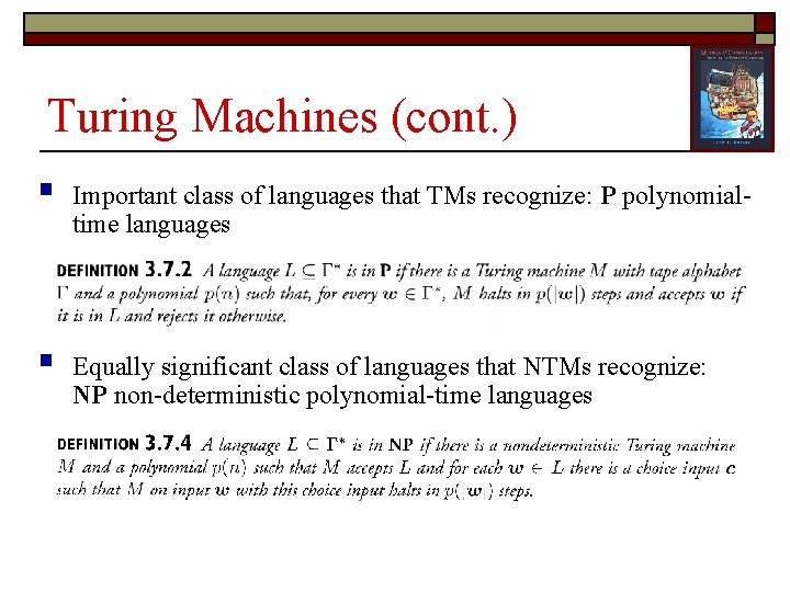
Turing Machines (cont. ) § Important class of languages that TMs recognize: P polynomialtime languages § Equally significant class of languages that NTMs recognize: NP non-deterministic polynomial-time languages

Turing Machines (cont. ) § § Languages in NP can be verified in a polynomial number of steps: a candidate string can be validated as member of the language in polynomial time Some problems that are in NP: n n n § Traveling Salesperson Problem (TSP) Graph 3 -Colorability (3 COL) Multiprocessor Scheduling (MSKED) Bin Packing (BNPAK) Crossword Puzzle Construction (CRSCON) It is not known whether P and NP include exactly the same set of problems, or one (NP) is larger than the other (P)

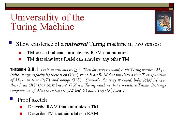
Universality of the Turing Machine § Show existence of a universal Turing machine in two senses: n n § TM exists that can simulate any RAM computation TM that simulates RAM can simulate any other TM Proof sketch n n Describe RAM that simulates a TM Describe TM that simulates a RAM

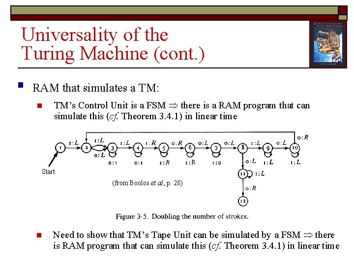
Universality of the Turing Machine (cont. ) § RAM that simulates a TM: n TM’s Control Unit is a FSM there is a RAM program that can simulate this (cf. Theorem 3. 4. 1) in linear time Start (from Boolos et al, p. 28) n Need to show that TM’s Tape Unit can be simulated by a FSM there is RAM program that can simulate this (cf. Theorem 3. 4. 1) in linear time

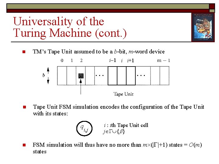
Universality of the Turing Machine (cont. ) n TM’s Tape Unit assumed to be a b-bit, m-word device i 1 i i+1 … n Tape Unit FSM simulation encodes the configuration of the Tape Unit with its states: q i, j n … i : ith Tape Unit cell j { } FSM simulation will thus have no more than m (| |+1) states = O(m) states

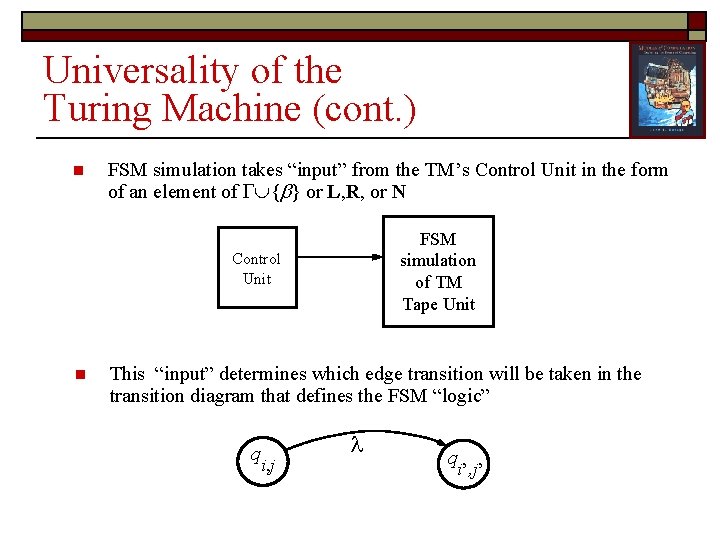
Universality of the Turing Machine (cont. ) n FSM simulation takes “input” from the TM’s Control Unit in the form of an element of { } or L, R, or N FSM simulation of TM Tape Unit Control Unit n This “input” determines which edge transition will be taken in the transition diagram that defines the FSM “logic” q i, j q i’, j’

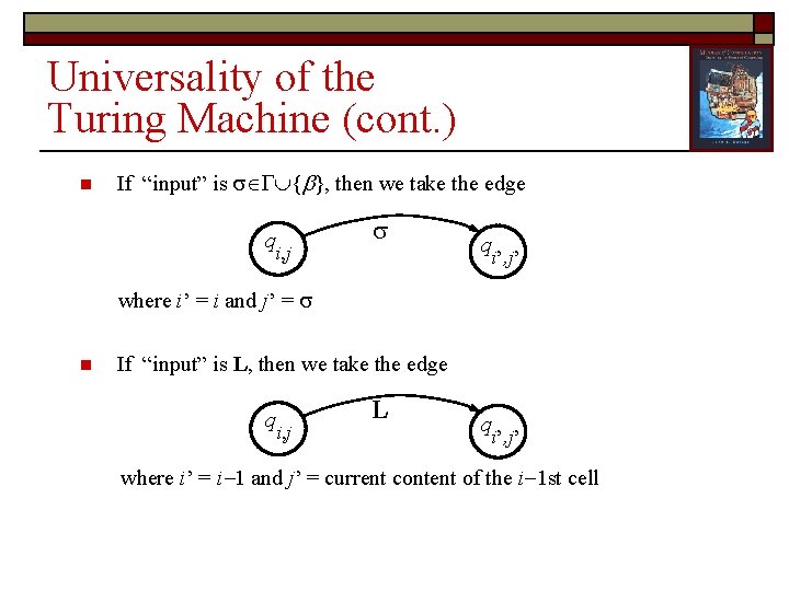
Universality of the Turing Machine (cont. ) n If “input” is { }, then we take the edge q i, j q i’, j’ where i’ = i and j’ = n If “input” is L, then we take the edge q i, j L q i’, j’ where i’ = i 1 and j’ = current content of the i 1 st cell

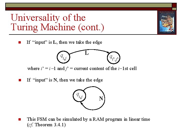
Universality of the Turing Machine (cont. ) n If “input” is L, then we take the edge L q i, j q i’, j’ where i’ = i 1 and j’ = current content of the i 1 st cell n If “input” is N, then we take the edge q i, j n N This FSM can be simulated by a RAM program in linear time (cf. Theorem 3. 4. 1)

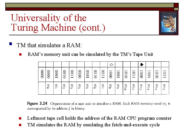
Universality of the Turing Machine (cont. ) § TM that simulates a RAM: n RAM’s memory unit can be simulated by the TM’s Tape Unit n Leftmost tape cell holds the address of the RAM CPU program counter TM simulates the RAM by emulating the fetch-and-execute cycle n

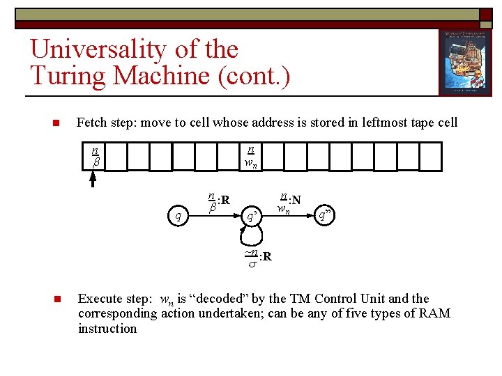
Universality of the Turing Machine (cont. ) n Fetch step: move to cell whose address is stored in leftmost tape cell n wn n n : R q q’ n : N wn q” ~n : R n Execute step: wn is “decoded” by the TM Control Unit and the corresponding action undertaken; can be any of five types of RAM instruction

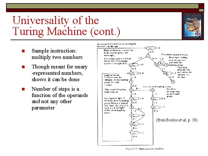
Universality of the Turing Machine (cont. ) n Sample instruction: multiply two numbers n Though meant for unary -represented numbers, shows it can be done n Number of steps is a function of the operands and not any other parameter (from Boolos et al, p. 30)

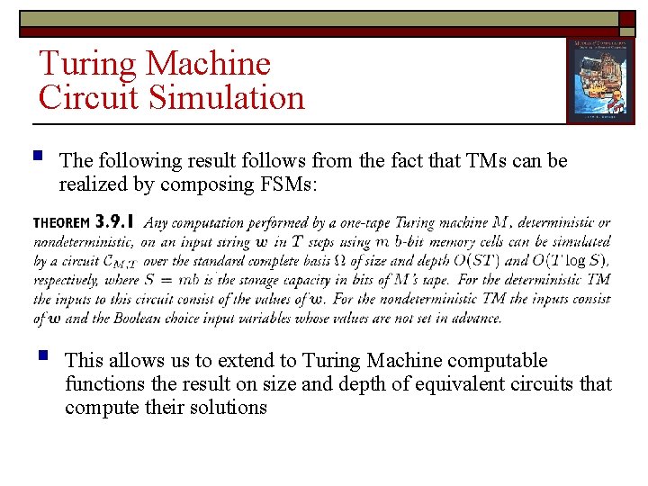
Turing Machine Circuit Simulation § The following result follows from the fact that TMs can be realized by composing FSMs: § This allows us to extend to Turing Machine computable functions the result on size and depth of equivalent circuits that compute their solutions

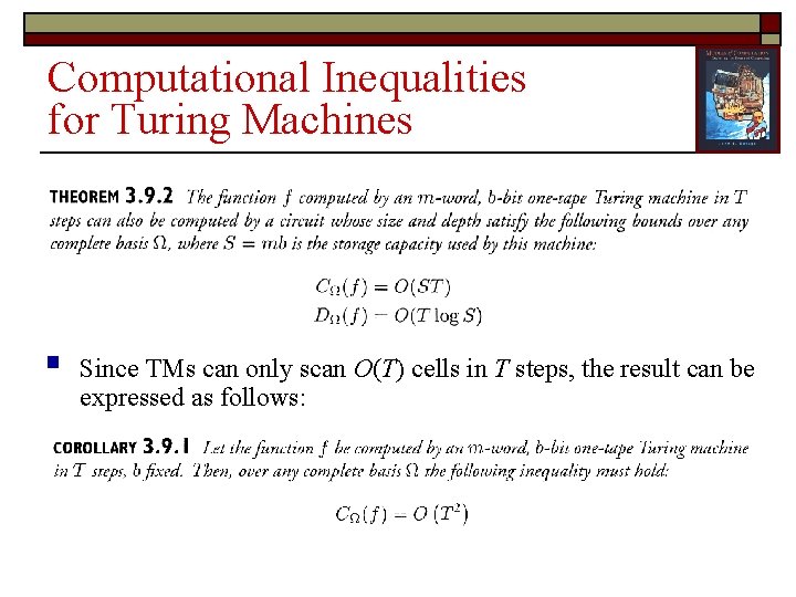
Computational Inequalities for Turing Machines § Since TMs can only scan O(T) cells in T steps, the result can be expressed as follows:

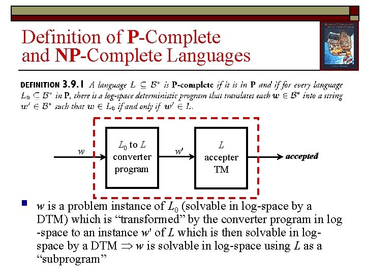
Definition of P-Complete and NP-Complete Languages w § L 0 to L converter program w' L accepter TM accepted w is a problem instance of L 0 (solvable in log-space by a DTM) which is “transformed” by the converter program in log -space to an instance w' of L which is then solvable in logspace by a DTM w is solvable in log-space using L as a “subprogram”

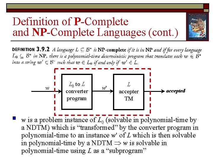
Definition of P-Complete and NP-Complete Languages (cont. ) w § L 0 to L converter program w' L accepter TM accepted w is a problem instance of L 0 (solvable in polynomial-time by a NDTM) which is “transformed” by the converter program in polynomial-time to an instance w' of L which is then solvable in polynomial-time by a NDTM w is solvable in polynomial-time using L as a “subprogram”

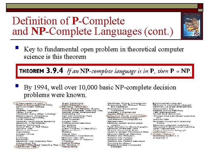
Definition of P-Complete and NP-Complete Languages (cont. ) § Key to fundamental open problem in theoretical computer science is theorem § By 1994, well over 10, 000 basic NP-complete decision problems were known.

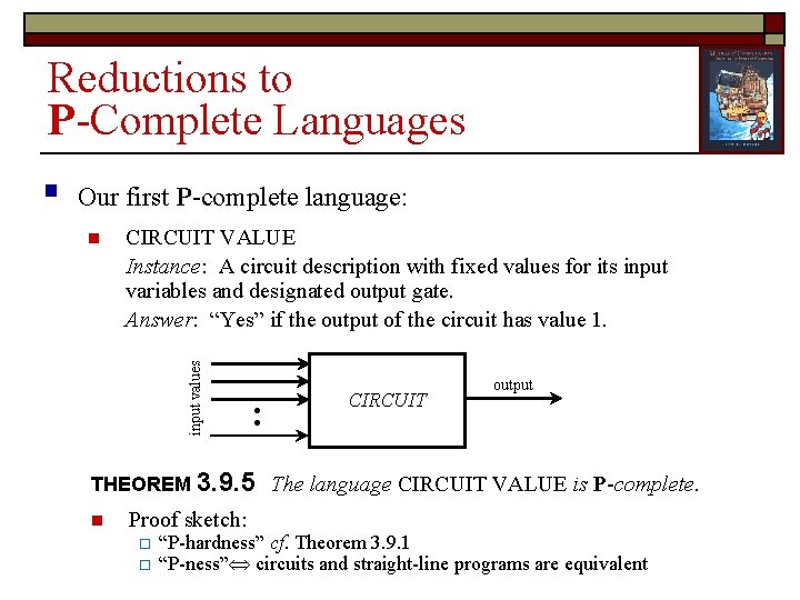
Reductions to P-Complete Languages Our first P-complete language: n CIRCUIT VALUE Instance: A circuit description with fixed values for its input variables and designated output gate. Answer: “Yes” if the output of the circuit has value 1. input values § : CIRCUIT output THEOREM 3. 9. 5 The language CIRCUIT VALUE is P-complete. n Proof sketch: o o “P-hardness” cf. Theorem 3. 9. 1 “P-ness” circuits and straight-line programs are equivalent

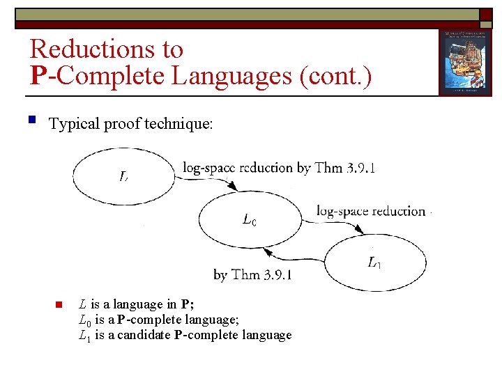
Reductions to P-Complete Languages (cont. ) § Typical proof technique: n L is a language in P; L 0 is a P-complete language; L 1 is a candidate P-complete language

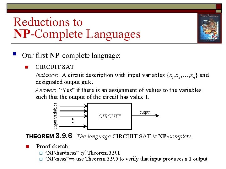
Reductions to NP-Complete Languages Our first NP-complete language: n CIRCUIT SAT Instance: A circuit description with input variables {x 1, x 2, …, xn} and designated output gate. Answer: “Yes” if there is an assignment of values to the variables such that the output of the circuit has value 1. input variables § : CIRCUIT output THEOREM 3. 9. 6 The language CIRCUIT SAT is NP-complete. n Proof sketch: o o “NP-hardness” cf. Theorem 3. 9. 1 “NP-ness” use Theorem 3. 9. 5 to verify that input produces a 1 output

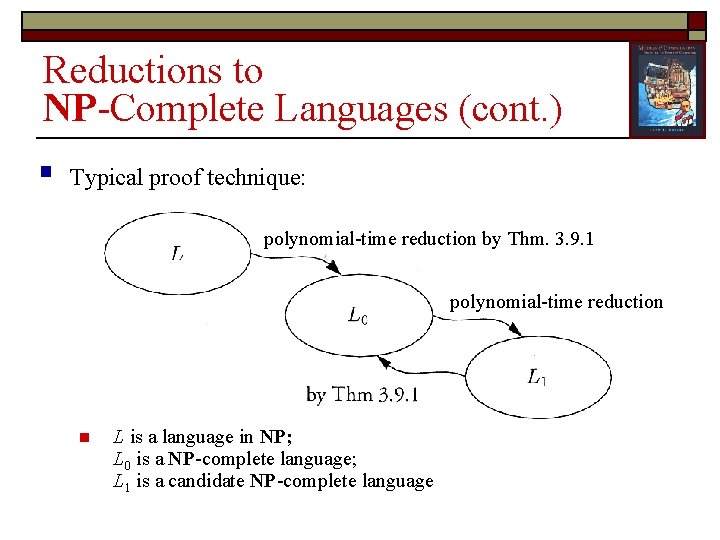
Reductions to NP-Complete Languages (cont. ) § Typical proof technique: polynomial-time reduction by Thm. 3. 9. 1 polynomial-time reduction n L is a language in NP; L 0 is a NP-complete language; L 1 is a candidate NP-complete language

Reductions to NP-Complete Languages (cont. ) § Our second NP-complete language: n SATISFIABILITY (SAT) Instance: A set of literals X={x 1, x 2, …, xn, xn} and a sequence of clauses C= {c 1, c 2, …, cm} where each clause ci is a subset of X. Answer: “Yes” if there is a (satisfying) assignment of values to the variables {x 1, x 2, …, xn} over the set B such that each clause has at least one literal whose value is 1. THEOREM 3. 9. 7 SATISFIABILITY is NP-complete. n Proof sketch: o o “NP-ness” can verify a “guess” in polynomial-time “NP-hardness” reduce CIRCUIT SAT to SAT

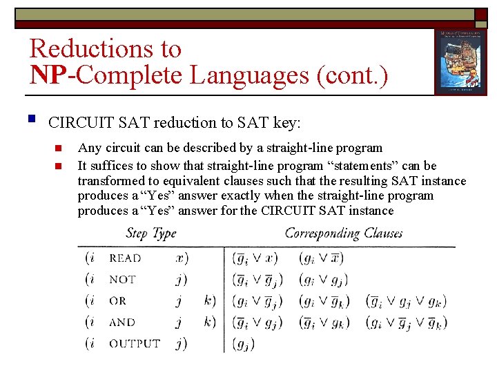
Reductions to NP-Complete Languages (cont. ) § CIRCUIT SAT reduction to SAT key: n n Any circuit can be described by a straight-line program It suffices to show that straight-line program “statements” can be transformed to equivalent clauses such that the resulting SAT instance produces a “Yes” answer exactly when the straight-line program produces a “Yes” answer for the CIRCUIT SAT instance