Machine Learning Structured Models Hidden Markov Models versus

Machine Learning Structured Models: Hidden Markov Models versus Conditional Random Fields Eric Xing Lecture 13, August 15, 2010 Reading: Eric Xing © Eric Xing @ CMU, 2006 -2010

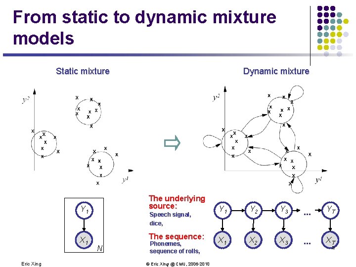
From static to dynamic mixture models Static mixture The underlying source: Y 1 A 1 X Eric Xing Dynamic mixture Speech signal, dice, The sequence: N Phonemes, sequence of rolls, © Eric Xing @ CMU, 2006 -2010 Y 1 Y 2 Y 3 . . . YT A 1 X A 2 X A 3 X . . . XAT 2

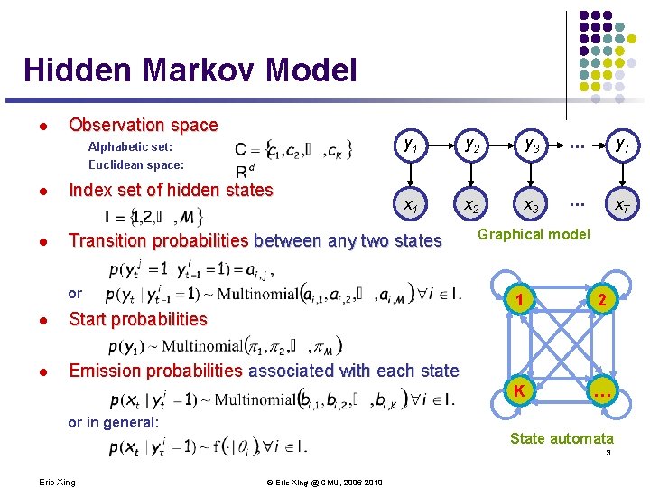
Hidden Markov Model l Observation space Alphabetic set: y 1 y 2 y 3 . . . y. T x. A 1 x. A 2 x. A 3 . . . x. AT Euclidean space: l Index set of hidden states l Transition probabilities between any two states or l Start probabilities l Emission probabilities associated with each state or in general: Graphical model 1 2 K … State automata 3 Eric Xing © Eric Xing @ CMU, 2006 -2010

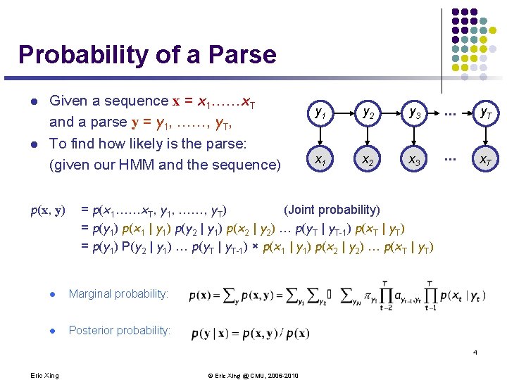
Probability of a Parse l l Given a sequence x = x 1……x. T and a parse y = y 1, ……, y. T, To find how likely is the parse: (given our HMM and the sequence) p(x, y) y 1 y 2 y 3 . . . y. T x. A 1 x. A 2 x. A 3 . . . x. AT = p(x 1……x. T, y 1, ……, y. T) (Joint probability) = p(y 1) p(x 1 | y 1) p(y 2 | y 1) p(x 2 | y 2) … p(y. T | y. T-1) p(x. T | y. T) = p(y 1) P(y 2 | y 1) … p(y. T | y. T-1) × p(x 1 | y 1) p(x 2 | y 2) … p(x. T | y. T) l Marginal probability: l Posterior probability: 4 Eric Xing © Eric Xing @ CMU, 2006 -2010

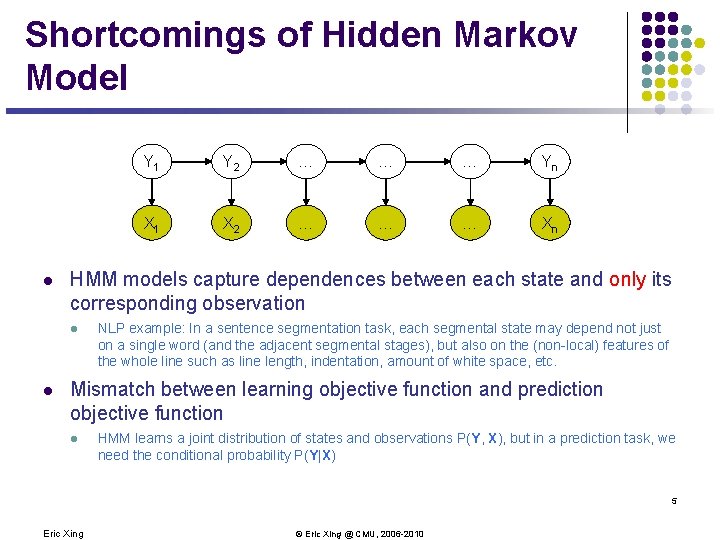
Shortcomings of Hidden Markov Model l Y 2 … … … Yn X 1 X 2 … … … Xn HMM models capture dependences between each state and only its corresponding observation l l Y 1 NLP example: In a sentence segmentation task, each segmental state may depend not just on a single word (and the adjacent segmental stages), but also on the (non-local) features of the whole line such as line length, indentation, amount of white space, etc. Mismatch between learning objective function and prediction objective function l HMM learns a joint distribution of states and observations P(Y, X), but in a prediction task, we need the conditional probability P(Y|X) 5 Eric Xing © Eric Xing @ CMU, 2006 -2010

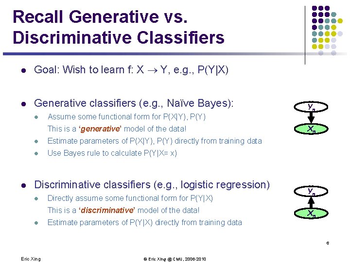
Recall Generative vs. Discriminative Classifiers l Goal: Wish to learn f: X ® Y, e. g. , P(Y|X) l Generative classifiers (e. g. , Naïve Bayes): l Assume some functional form for P(X|Y), P(Y) This is a ‘generative’ model of the data! l l Estimate parameters of P(X|Y), P(Y) directly from training data l Use Bayes rule to calculate P(Y|X= x) Discriminative classifiers (e. g. , logistic regression) l Directly assume some functional form for P(Y|X) This is a ‘discriminative’ model of the data! l Estimate parameters of P(Y|X) directly from training data Yn Xn 6 Eric Xing © Eric Xing @ CMU, 2006 -2010

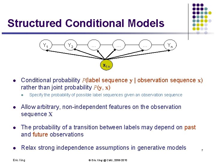
Structured Conditional Models Y 1 Y 2 … … … Yn x 1: n l Conditional probability P(label sequence y | observation sequence x) rather than joint probability P(y, x) l Specify the probability of possible label sequences given an observation sequence l Allow arbitrary, non-independent features on the observation sequence X l The probability of a transition between labels may depend on past and future observations l Relax strong independence assumptions in generative models Eric Xing © Eric Xing @ CMU, 2006 -2010 7

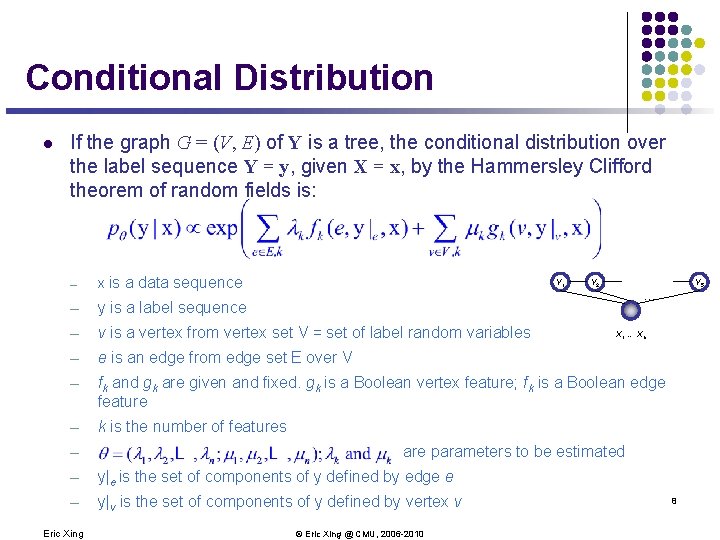
Conditional Distribution l If the graph G = (V, E) of Y is a tree, the conditional distribution over the label sequence Y = y, given X = x, by the Hammersley Clifford theorem of random fields is: ─ x is a data sequence ─ y is a label sequence ─ v is a vertex from vertex set V = set of label random variables ─ e is an edge from edge set E over V ─ fk and gk are given and fixed. gk is a Boolean vertex feature; fk is a Boolean edge feature ─ k is the number of features ─ Y 1 Y 5 … X 1 … Xn are parameters to be estimated ─ y|e is the set of components of y defined by edge e ─ y|v is the set of components of y defined by vertex v Eric Xing Y 2 © Eric Xing @ CMU, 2006 -2010 8

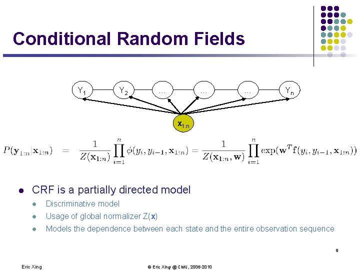
Conditional Random Fields Y 1 Y 2 … … … Yn x 1: n l CRF is a partially directed model l Discriminative model l Usage of global normalizer Z(x) l Models the dependence between each state and the entire observation sequence 9 Eric Xing © Eric Xing @ CMU, 2006 -2010

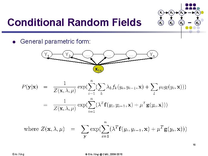
Conditional Random Fields l General parametric form: Y 1 Y 2 … … … Yn x 1: n 10 Eric Xing © Eric Xing @ CMU, 2006 -2010

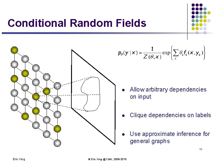
Conditional Random Fields l Allow arbitrary dependencies on input l Clique dependencies on labels l Use approximate inference for general graphs 11 Eric Xing © Eric Xing @ CMU, 2006 -2010

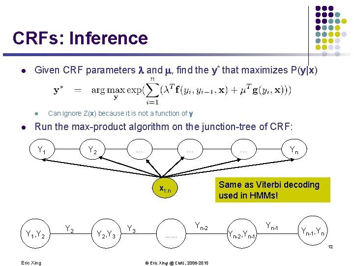
CRFs: Inference l Given CRF parameters and , find the y* that maximizes P(y|x) l l Can ignore Z(x) because it is not a function of y Run the max-product algorithm on the junction-tree of CRF: Y 1 Y 2 … … … Same as Viterbi decoding used in HMMs! x 1: n Y 1, Y 2 Y 2, Y 3 Yn Yn-2 ……. Yn-2, Yn-1, Yn 12 Eric Xing © Eric Xing @ CMU, 2006 -2010

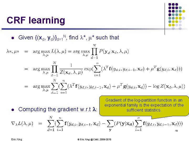
CRF learning l l Given {(xd, yd)}d=1 N, find *, * such that Computing the gradient w. r. t : Gradient of the log-partition function in an exponential family is the expectation of the sufficient statistics. 13 Eric Xing © Eric Xing @ CMU, 2006 -2010

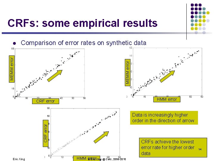
CRFs: some empirical results Comparison of error rates on synthetic data MEMM error l HMM error CRF error Data is increasingly higher order in the direction of arrow Eric Xing CRFs achieve the lowest error rate for higher order data HMM error © Eric Xing @ CMU, 2006 -2010 14

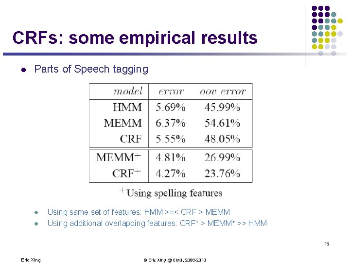
CRFs: some empirical results l Parts of Speech tagging l l Using same set of features: HMM >=< CRF > MEMM Using additional overlapping features: CRF+ > MEMM+ >> HMM 15 Eric Xing © Eric Xing @ CMU, 2006 -2010

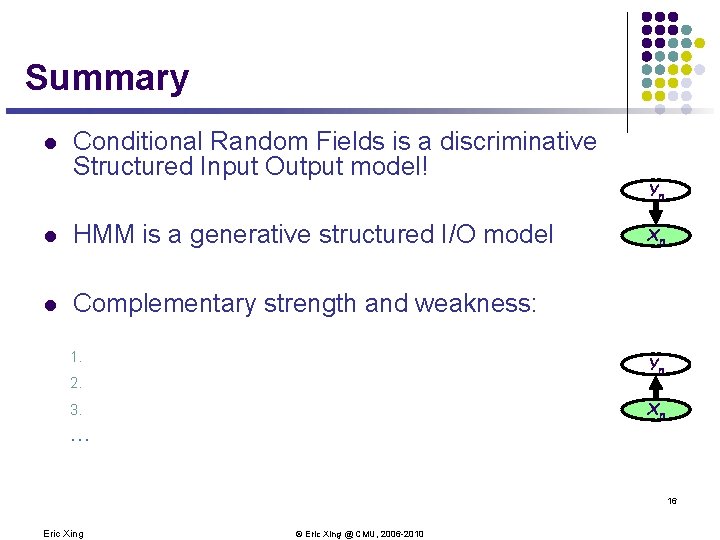
Summary l Conditional Random Fields is a discriminative Structured Input Output model! l HMM is a generative structured I/O model l Complementary strength and weakness: 1. Yn Xn Yn 2. Xn 3. … 16 Eric Xing © Eric Xing @ CMU, 2006 -2010