Machine Learning Structured Models Hidden Markov Models versus

Machine Learning Structured Models: Hidden Markov Models versus Conditional Random Fields Eric Xing Lecture 13, August 15, 2010 Reading: Eric Xing © Eric Xing @ CMU, 2006 -2010

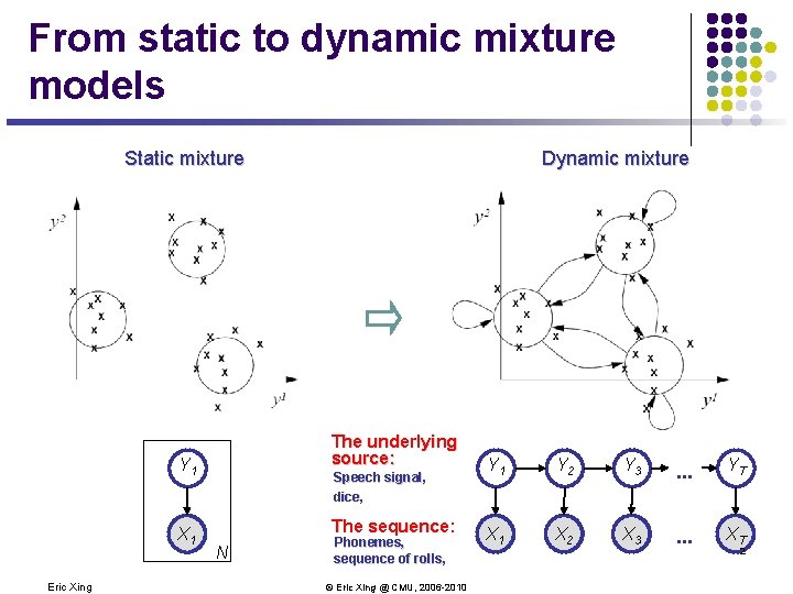
From static to dynamic mixture models Static mixture The underlying source: Y 1 A 1 X Eric Xing Dynamic mixture Speech signal, dice, The sequence: N Phonemes, sequence of rolls, © Eric Xing @ CMU, 2006 -2010 Y 1 Y 2 Y 3 . . . YT A 1 X A 2 X A 3 X . . . XAT 2

Predicting Tumor Cell States Chromosomes of tumor cell: 3 Eric Xing © Eric Xing @ CMU, 2006 -2010

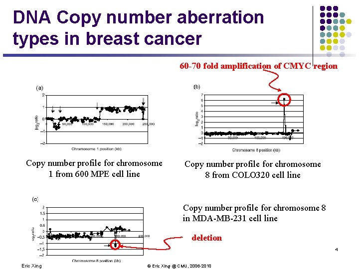
DNA Copy number aberration types in breast cancer 60 -70 fold amplification of CMYC region Copy number profile for chromosome 1 from 600 MPE cell line Copy number profile for chromosome 8 from COLO 320 cell line Copy number profile for chromosome 8 in MDA-MB-231 cell line deletion 4 Eric Xing © Eric Xing @ CMU, 2006 -2010

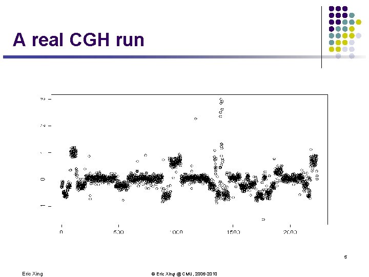
A real CGH run 5 Eric Xing © Eric Xing @ CMU, 2006 -2010

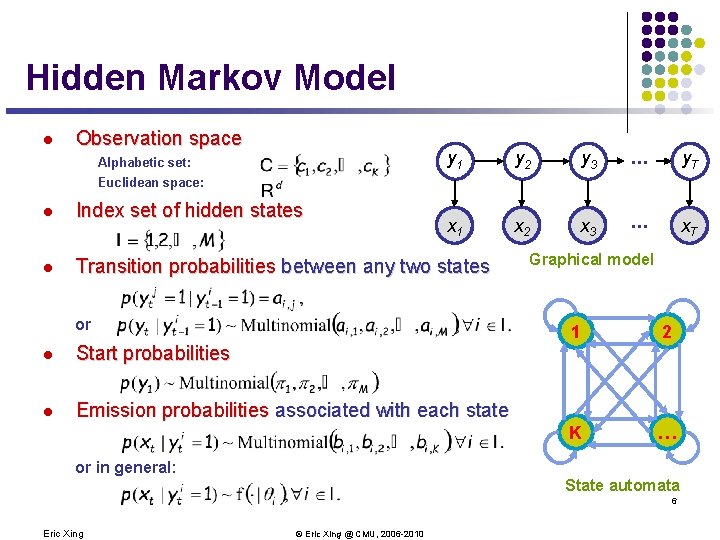
Hidden Markov Model l Observation space Alphabetic set: y 1 y 2 y 3 . . . y. T x. A 1 x. A 2 x. A 3 . . . x. AT Euclidean space: l Index set of hidden states l Transition probabilities between any two states or l Start probabilities l Emission probabilities associated with each state or in general: Graphical model 1 2 K … State automata 6 Eric Xing © Eric Xing @ CMU, 2006 -2010

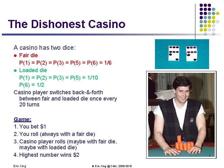
The Dishonest Casino A casino has two dice: Fair die P(1) = P(2) = P(3) = P(5) = P(6) = 1/6 l Loaded die P(1) = P(2) = P(3) = P(5) = 1/10 P(6) = 1/2 Casino player switches back-&-forth between fair and loaded die once every 20 turns l Game: 1. You bet $1 2. You roll (always with a fair die) 3. Casino player rolls (maybe with fair die, maybe with loaded die) 4. Highest number wins $2 Eric Xing © Eric Xing @ CMU, 2006 -2010 7

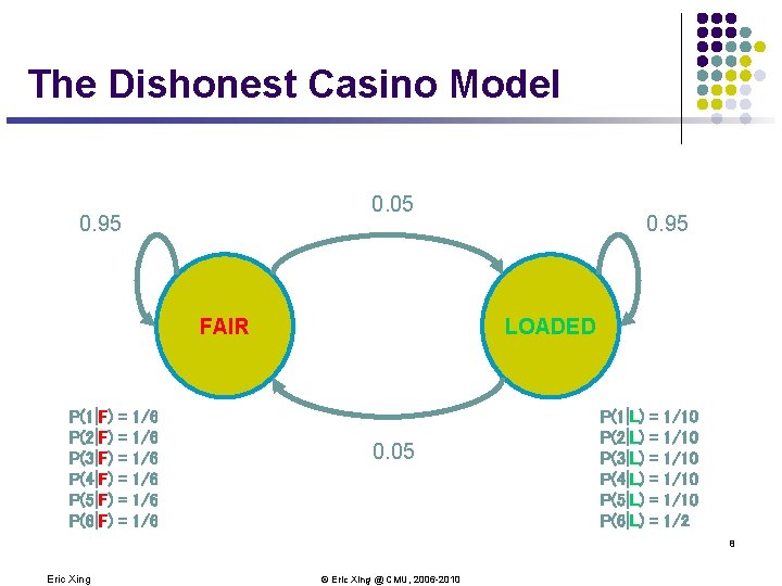
The Dishonest Casino Model 0. 05 0. 95 FAIR P(1|F) P(2|F) P(3|F) P(4|F) P(5|F) P(6|F) = = = 1/6 1/6 1/6 0. 95 LOADED 0. 05 P(1|L) P(2|L) P(3|L) P(4|L) P(5|L) P(6|L) = = = 1/10 1/10 1/2 8 Eric Xing © Eric Xing @ CMU, 2006 -2010

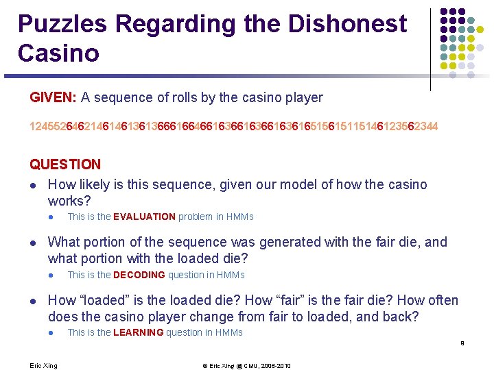
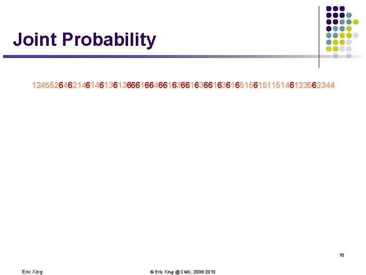
Puzzles Regarding the Dishonest Casino GIVEN: A sequence of rolls by the casino player 12455264621461461361366616646616366163616515615115146123562344 QUESTION l How likely is this sequence, given our model of how the casino works? l l What portion of the sequence was generated with the fair die, and what portion with the loaded die? l l This is the EVALUATION problem in HMMs This is the DECODING question in HMMs How “loaded” is the loaded die? How “fair” is the fair die? How often does the casino player change from fair to loaded, and back? l This is the LEARNING question in HMMs 9 Eric Xing © Eric Xing @ CMU, 2006 -2010

Joint Probability 12455264621461461361366616646616366163616515615115146123562344 10 Eric Xing © Eric Xing @ CMU, 2006 -2010

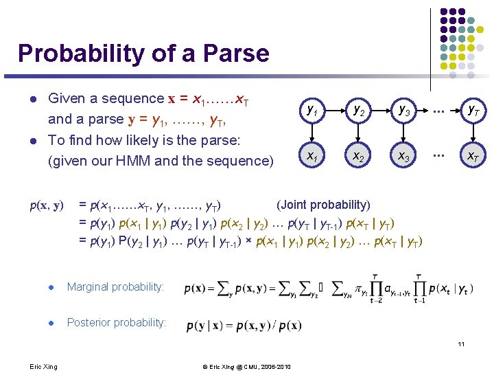
Probability of a Parse l l Given a sequence x = x 1……x. T and a parse y = y 1, ……, y. T, To find how likely is the parse: (given our HMM and the sequence) p(x, y) y 1 y 2 y 3 . . . y. T x. A 1 x. A 2 x. A 3 . . . x. AT = p(x 1……x. T, y 1, ……, y. T) (Joint probability) = p(y 1) p(x 1 | y 1) p(y 2 | y 1) p(x 2 | y 2) … p(y. T | y. T-1) p(x. T | y. T) = p(y 1) P(y 2 | y 1) … p(y. T | y. T-1) × p(x 1 | y 1) p(x 2 | y 2) … p(x. T | y. T) l Marginal probability: l Posterior probability: 11 Eric Xing © Eric Xing @ CMU, 2006 -2010

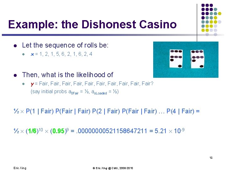
Example: the Dishonest Casino l Let the sequence of rolls be: l l x = 1, 2, 1, 5, 6, 2, 1, 6, 2, 4 Then, what is the likelihood of l y = Fair, Fair, Fair, Fair? (say initial probs a 0 Fair = ½, ao. Loaded = ½) ½ P(1 | Fair) P(Fair | Fair) P(2 | Fair) P(Fair | Fair) … P(4 | Fair) = ½ (1/6)10 (0. 95)9 =. 0000521158647211 = 5. 21 10 -9 12 Eric Xing © Eric Xing @ CMU, 2006 -2010

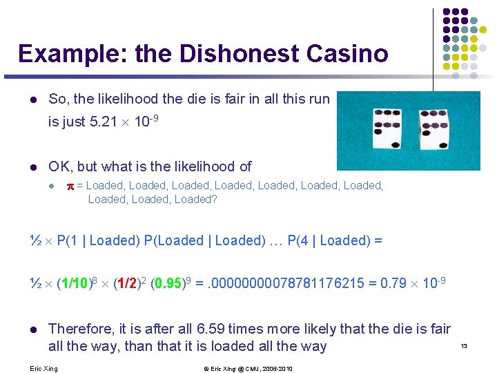
Example: the Dishonest Casino l So, the likelihood the die is fair in all this run is just 5. 21 10 -9 l OK, but what is the likelihood of l = Loaded, Loaded, Loaded, Loaded? ½ P(1 | Loaded) P(Loaded | Loaded) … P(4 | Loaded) = ½ (1/10)8 (1/2)2 (0. 95)9 =. 0000078781176215 = 0. 79 10 -9 l Therefore, it is after all 6. 59 times more likely that the die is fair all the way, than that it is loaded all the way Eric Xing © Eric Xing @ CMU, 2006 -2010 13

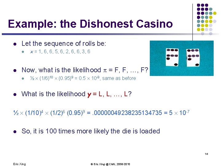
Example: the Dishonest Casino l Let the sequence of rolls be: l l Now, what is the likelihood = F, F, …, F? l l x = 1, 6, 6, 5, 6, 2, 6, 6, 3, 6 ½ (1/6)10 (0. 95)9 = 0. 5 10 -9, same as before What is the likelihood y = L, L, …, L? ½ (1/10)4 (1/2)6 (0. 95)9 =. 00000049238235134735 = 5 10 -7 l So, it is 100 times more likely the die is loaded 14 Eric Xing © Eric Xing @ CMU, 2006 -2010

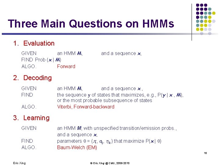
Three Main Questions on HMMs 1. Evaluation GIVEN an HMM M, FIND Prob (x | M) ALGO. Forward and a sequence x, 2. Decoding GIVEN FIND ALGO. an HMM M, and a sequence x , the sequence y of states that maximizes, e. g. , P(y | x , M), or the most probable subsequence of states Viterbi, Forward-backward 3. Learning GIVEN FIND ALGO. an HMM M, with unspecified transition/emission probs. , and a sequence x, parameters = (pi, aij, hik) that maximize P(x | ) Baum-Welch (EM) 15 Eric Xing © Eric Xing @ CMU, 2006 -2010

Applications of HMMs l Some early applications of HMMs l finance, but we never saw them l speech recognition l modelling ion channels l In the mid-late 1980 s HMMs entered genetics and molecular biology, and they are now firmly entrenched. l Some current applications of HMMs to biology l mapping chromosomes l aligning biological sequences l predicting sequence structure l inferring evolutionary relationships l finding genes in DNA sequence 16 Eric Xing © Eric Xing @ CMU, 2006 -2010

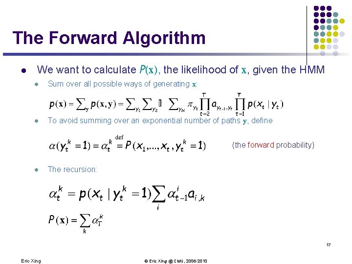
The Forward Algorithm l We want to calculate P(x), the likelihood of x, given the HMM l Sum over all possible ways of generating x: l To avoid summing over an exponential number of paths y, define (the forward probability) l The recursion: 17 Eric Xing © Eric Xing @ CMU, 2006 -2010

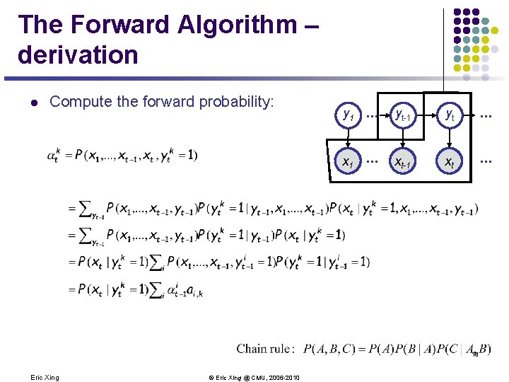
The Forward Algorithm – derivation l Compute the forward probability: y 1 . . . yt-1 yt . . . x. A 1 . . . x. A t-1 xt A . . . 18 Eric Xing © Eric Xing @ CMU, 2006 -2010

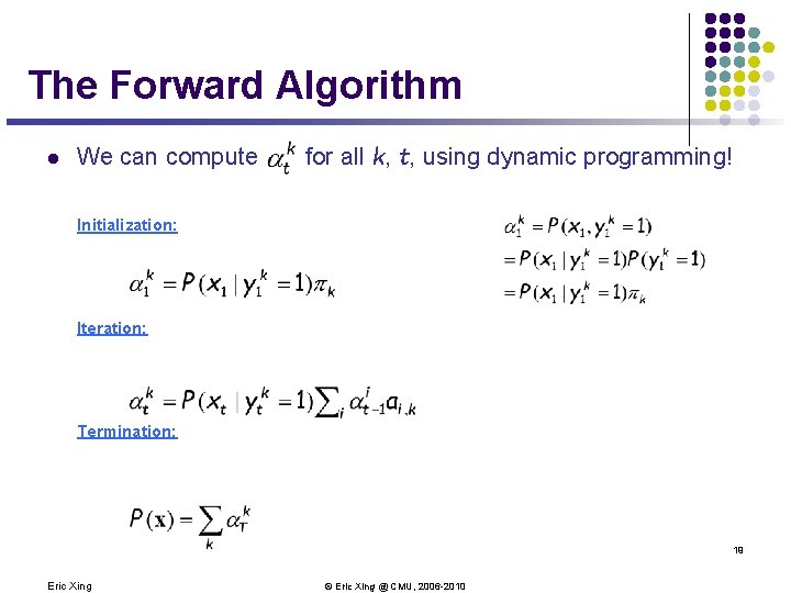
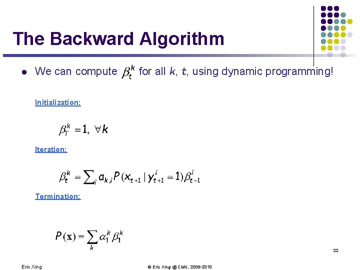
The Forward Algorithm l We can compute for all k, t, using dynamic programming! Initialization: Iteration: Termination: 19 Eric Xing © Eric Xing @ CMU, 2006 -2010

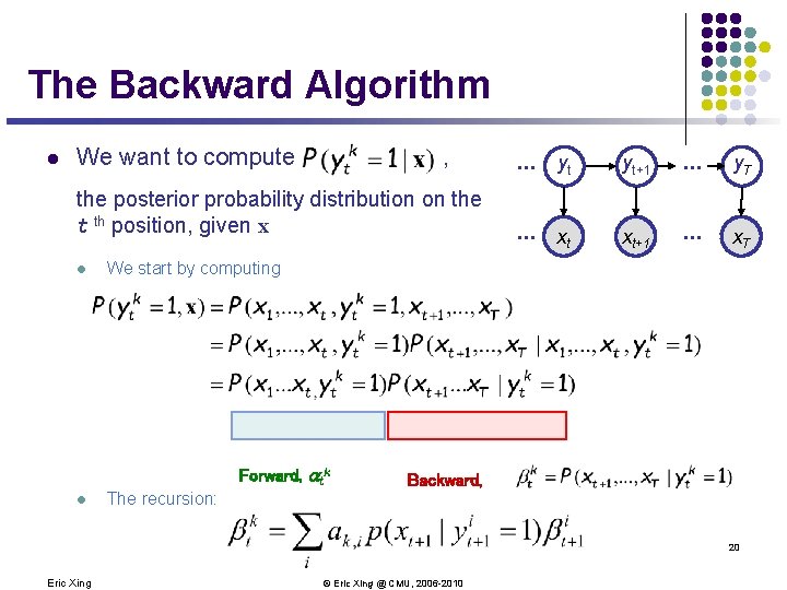
The Backward Algorithm l We want to compute , the posterior probability distribution on the t th position, given x l yt yt+1 . . . y. T . . . A xt x. A t+1 . . . x. AT We start by computing Forward, atk l . . . Backward, The recursion: 20 Eric Xing © Eric Xing @ CMU, 2006 -2010

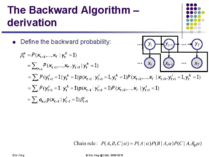
The Backward Algorithm – derivation l Define the backward probability: . . . yt yt+1 . . . y. T . . . A xt x. A t+1 . . . x. AT 21 Eric Xing © Eric Xing @ CMU, 2006 -2010

The Backward Algorithm l We can compute for all k, t, using dynamic programming! Initialization: Iteration: Termination: 22 Eric Xing © Eric Xing @ CMU, 2006 -2010

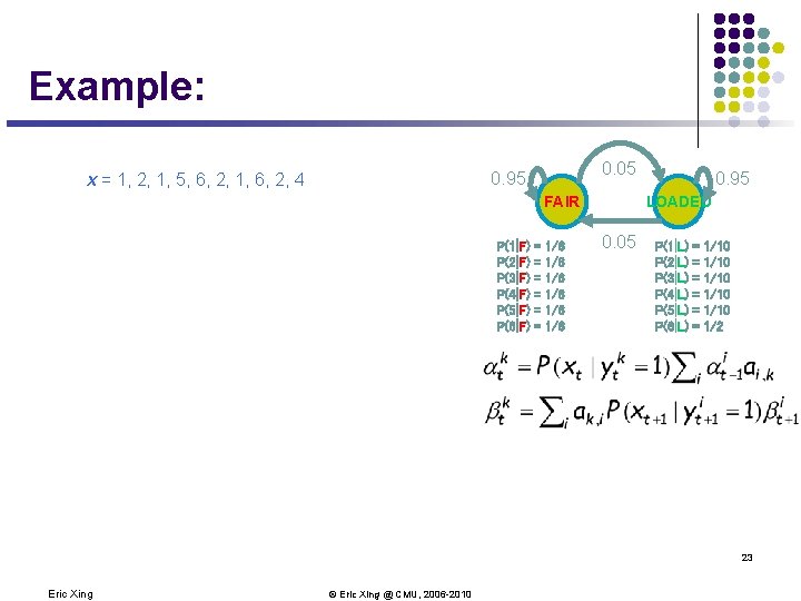
Example: 0. 05 0. 95 x = 1, 2, 1, 5, 6, 2, 1, 6, 2, 4 FAIR P(1|F) P(2|F) P(3|F) P(4|F) P(5|F) P(6|F) = = = 1/6 1/6 1/6 0. 95 LOADED 0. 05 P(1|L) P(2|L) P(3|L) P(4|L) P(5|L) P(6|L) = = = 1/10 1/10 1/2 23 Eric Xing © Eric Xing @ CMU, 2006 -2010

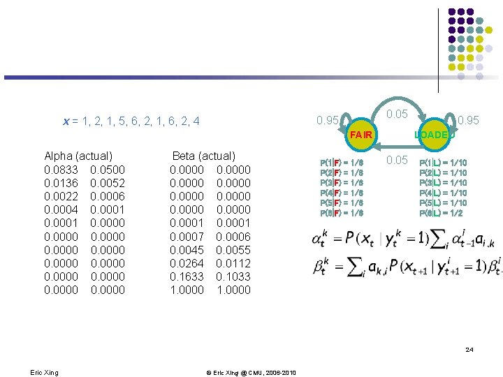
0. 05 0. 95 x = 1, 2, 1, 5, 6, 2, 1, 6, 2, 4 FAIR Alpha (actual) 0. 0833 0. 0500 0. 0136 0. 0052 0. 0022 0. 0006 0. 0004 0. 0001 0. 0000 0. 0000 Beta (actual) 0. 0000 0. 0001 0. 0007 0. 0006 0. 0045 0. 0055 0. 0264 0. 0112 0. 1633 0. 1033 1. 0000 P(1|F) P(2|F) P(3|F) P(4|F) P(5|F) P(6|F) = = = 1/6 1/6 1/6 0. 95 LOADED 0. 05 P(1|L) P(2|L) P(3|L) P(4|L) P(5|L) P(6|L) = = = 1/10 1/10 1/2 24 Eric Xing © Eric Xing @ CMU, 2006 -2010

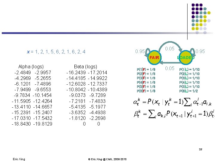
0. 05 0. 95 x = 1, 2, 1, 5, 6, 2, 1, 6, 2, 4 FAIR Alpha (logs) -2. 4849 -2. 9957 -4. 2969 -5. 2655 -6. 1201 -7. 4896 -7. 9499 -9. 6553 -9. 7834 -10. 1454 -11. 5905 -12. 4264 -13. 4110 -14. 6657 -15. 2391 -15. 2407 -17. 0310 -17. 5432 -18. 8430 -19. 8129 Beta (logs) -16. 2439 -17. 2014 -14. 4185 -14. 9922 -12. 6028 -12. 7337 -10. 8042 -10. 4389 -9. 0373 -9. 7289 -7. 2181 -7. 4833 -5. 4135 -5. 1977 -3. 6352 -4. 4938 -1. 8120 -2. 2698 0 0 P(1|F) P(2|F) P(3|F) P(4|F) P(5|F) P(6|F) = = = 1/6 1/6 1/6 0. 95 LOADED 0. 05 P(1|L) P(2|L) P(3|L) P(4|L) P(5|L) P(6|L) = = = 1/10 1/10 1/2 25 Eric Xing © Eric Xing @ CMU, 2006 -2010

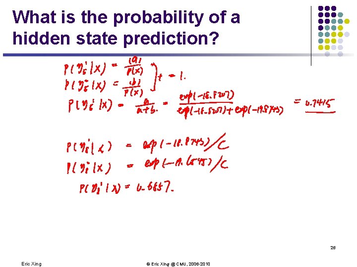
What is the probability of a hidden state prediction? 26 Eric Xing © Eric Xing @ CMU, 2006 -2010

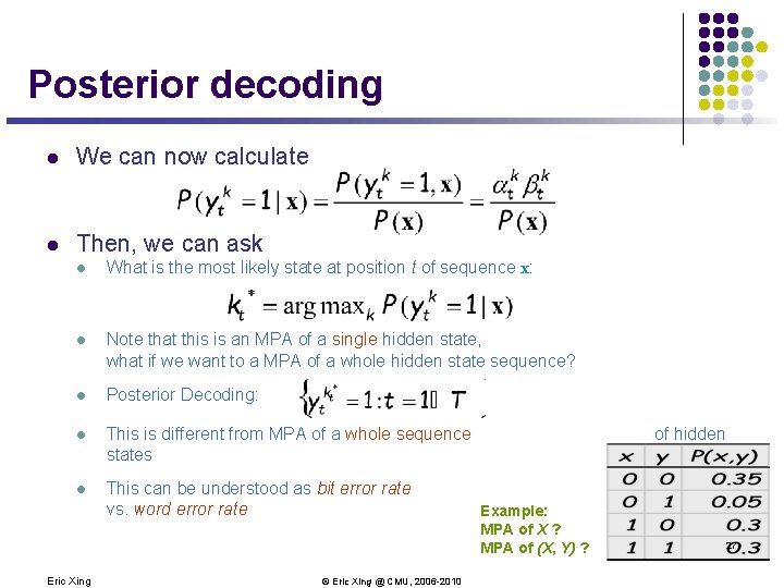
Posterior decoding l We can now calculate l Then, we can ask l What is the most likely state at position t of sequence x: l Note that this is an MPA of a single hidden state, what if we want to a MPA of a whole hidden state sequence? l Posterior Decoding: l This is different from MPA of a whole sequence states l This can be understood as bit error rate vs. word error rate Eric Xing © Eric Xing @ CMU, 2006 -2010 of hidden Example: MPA of X ? MPA of (X, Y) ? 27

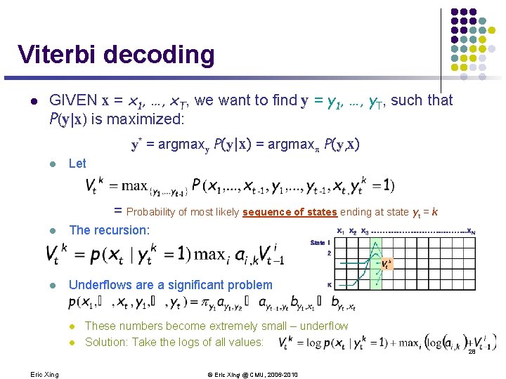
Viterbi decoding l GIVEN x = x 1, …, x. T, we want to find y = y 1, …, y. T, such that P(y|x) is maximized: y* = argmaxy P(y|x) = argmax P(y, x) l Let = Probability of most likely sequence of states ending at state yt = k l The recursion: l Underflows are a significant problem l l These numbers become extremely small – underflow Solution: Take the logs of all values: 28 Eric Xing © Eric Xing @ CMU, 2006 -2010

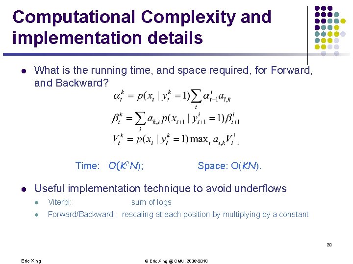
Computational Complexity and implementation details l What is the running time, and space required, for Forward, and Backward? Time: O(K 2 N); l Space: O(KN). Useful implementation technique to avoid underflows l Viterbi: sum of logs l Forward/Backward: rescaling at each position by multiplying by a constant 29 Eric Xing © Eric Xing @ CMU, 2006 -2010

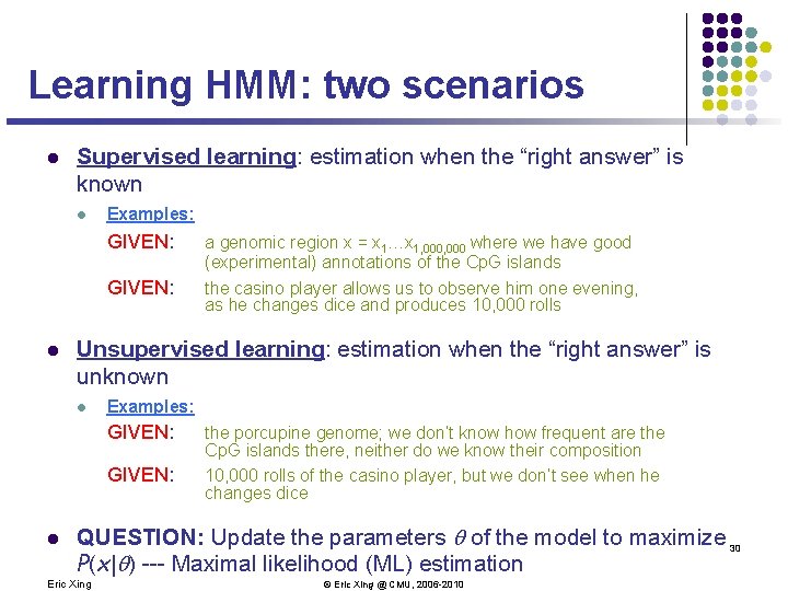
Learning HMM: two scenarios l Supervised learning: estimation when the “right answer” is known l Examples: GIVEN: l Unsupervised learning: estimation when the “right answer” is unknown l Examples: GIVEN: l a genomic region x = x 1…x 1, 000 where we have good (experimental) annotations of the Cp. G islands the casino player allows us to observe him one evening, as he changes dice and produces 10, 000 rolls the porcupine genome; we don’t know how frequent are the Cp. G islands there, neither do we know their composition 10, 000 rolls of the casino player, but we don’t see when he changes dice QUESTION: Update the parameters of the model to maximize 30 P(x| ) --- Maximal likelihood (ML) estimation Eric Xing © Eric Xing @ CMU, 2006 -2010

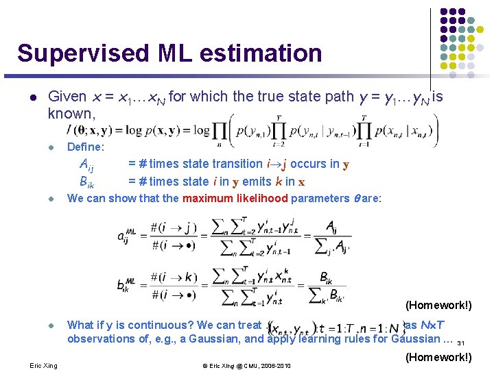
Supervised ML estimation l Given x = x 1…x. N for which the true state path y = y 1…y. N is known, l Define: Aij Bik l = # times state transition i j occurs in y = # times state i in y emits k in x We can show that the maximum likelihood parameters are: (Homework!) l Eric Xing What if y is continuous? We can treat as N´T observations of, e. g. , a Gaussian, and apply learning rules for Gaussian … 31 © Eric Xing @ CMU, 2006 -2010 (Homework!)

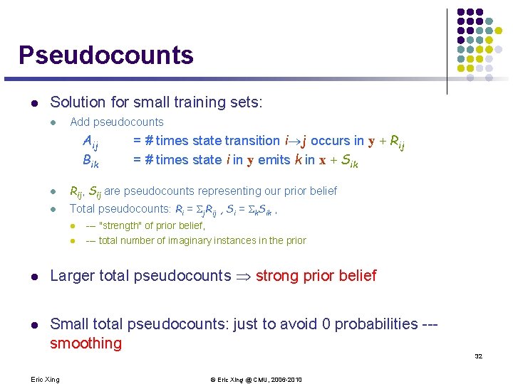
Pseudocounts l Solution for small training sets: l Add pseudocounts Aij Bik = # times state transition i j occurs in y + Rij = # times state i in y emits k in x + Sik l Rij, Sij are pseudocounts representing our prior belief l Total pseudocounts: Ri = Sj. Rij , Si = Sk. Sik , l --- "strength" of prior belief, l --- total number of imaginary instances in the prior l Larger total pseudocounts strong prior belief l Small total pseudocounts: just to avoid 0 probabilities --smoothing 32 Eric Xing © Eric Xing @ CMU, 2006 -2010

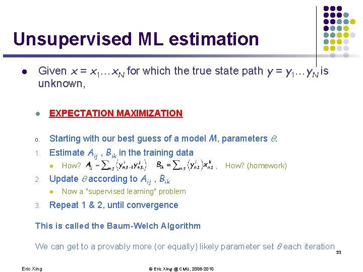
Unsupervised ML estimation l Given x = x 1…x. N for which the true state path y = y 1…y. N is unknown, l EXPECTATION MAXIMIZATION 0. Starting with our best guess of a model M, parameters : 1. Estimate Aij , Bik in the training data l 2. , , How? (homework) Update according to Aij , Bik l 3. How? Now a "supervised learning" problem Repeat 1 & 2, until convergence This is called the Baum-Welch Algorithm We can get to a provably more (or equally) likely parameter set each iteration Eric Xing © Eric Xing @ CMU, 2006 -2010 33

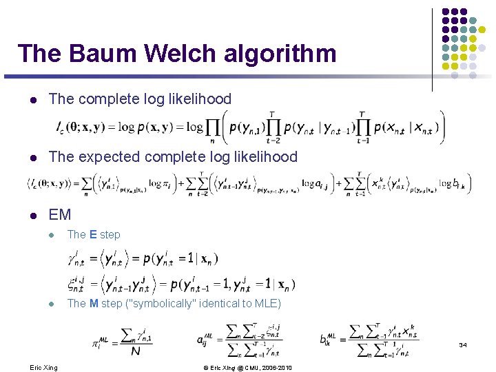
The Baum Welch algorithm l The complete log likelihood l The expected complete log likelihood l EM l The E step l The M step ("symbolically" identical to MLE) 34 Eric Xing © Eric Xing @ CMU, 2006 -2010

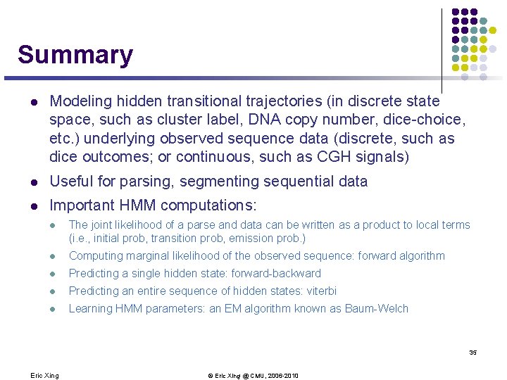
Summary l Modeling hidden transitional trajectories (in discrete state space, such as cluster label, DNA copy number, dice-choice, etc. ) underlying observed sequence data (discrete, such as dice outcomes; or continuous, such as CGH signals) l Useful for parsing, segmenting sequential data l Important HMM computations: l The joint likelihood of a parse and data can be written as a product to local terms (i. e. , initial prob, transition prob, emission prob. ) l Computing marginal likelihood of the observed sequence: forward algorithm l Predicting a single hidden state: forward-backward l Predicting an entire sequence of hidden states: viterbi l Learning HMM parameters: an EM algorithm known as Baum-Welch 35 Eric Xing © Eric Xing @ CMU, 2006 -2010

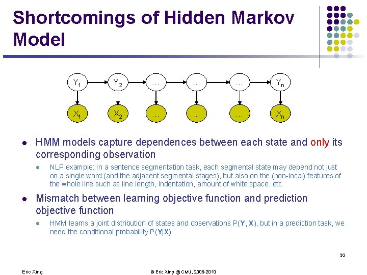
Shortcomings of Hidden Markov Model l Y 2 … … … Yn X 1 X 2 … … … Xn HMM models capture dependences between each state and only its corresponding observation l l Y 1 NLP example: In a sentence segmentation task, each segmental state may depend not just on a single word (and the adjacent segmental stages), but also on the (non-local) features of the whole line such as line length, indentation, amount of white space, etc. Mismatch between learning objective function and prediction objective function l HMM learns a joint distribution of states and observations P(Y, X), but in a prediction task, we need the conditional probability P(Y|X) 36 Eric Xing © Eric Xing @ CMU, 2006 -2010

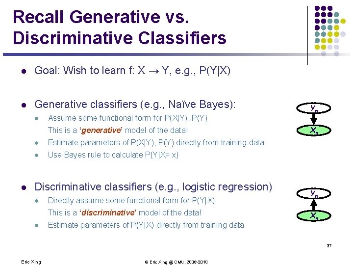
Recall Generative vs. Discriminative Classifiers l Goal: Wish to learn f: X Y, e. g. , P(Y|X) l Generative classifiers (e. g. , Naïve Bayes): l Assume some functional form for P(X|Y), P(Y) This is a ‘generative’ model of the data! l l Estimate parameters of P(X|Y), P(Y) directly from training data l Use Bayes rule to calculate P(Y|X= x) Discriminative classifiers (e. g. , logistic regression) l Directly assume some functional form for P(Y|X) This is a ‘discriminative’ model of the data! l Estimate parameters of P(Y|X) directly from training data Yn Xn 37 Eric Xing © Eric Xing @ CMU, 2006 -2010

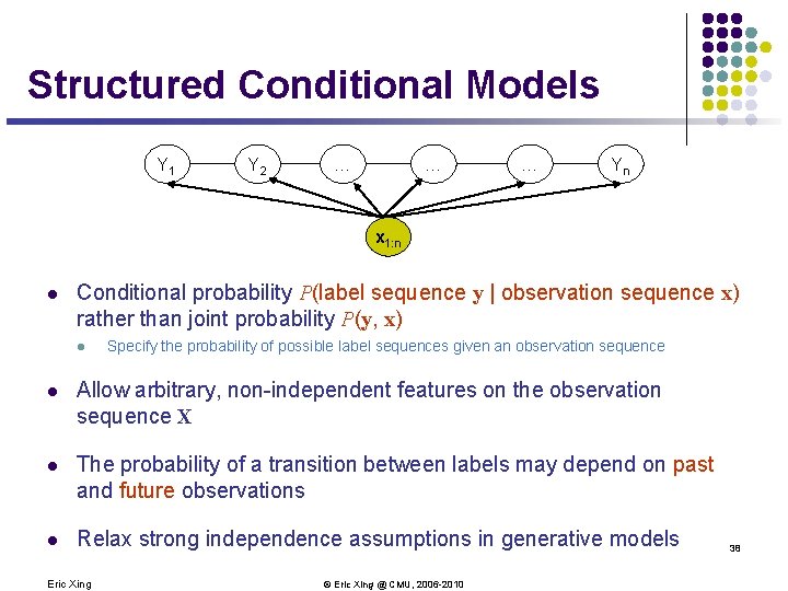
Structured Conditional Models Y 1 Y 2 … … … Yn x 1: n l Conditional probability P(label sequence y | observation sequence x) rather than joint probability P(y, x) l Specify the probability of possible label sequences given an observation sequence l Allow arbitrary, non-independent features on the observation sequence X l The probability of a transition between labels may depend on past and future observations l Relax strong independence assumptions in generative models Eric Xing © Eric Xing @ CMU, 2006 -2010 38

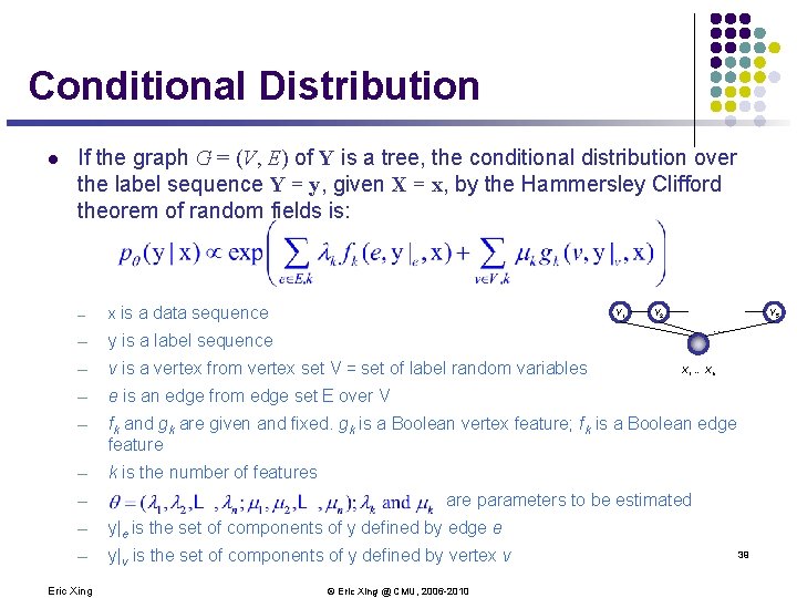
Conditional Distribution l If the graph G = (V, E) of Y is a tree, the conditional distribution over the label sequence Y = y, given X = x, by the Hammersley Clifford theorem of random fields is: ─ x is a data sequence ─ y is a label sequence ─ v is a vertex from vertex set V = set of label random variables ─ e is an edge from edge set E over V ─ fk and gk are given and fixed. gk is a Boolean vertex feature; fk is a Boolean edge feature ─ k is the number of features ─ Y 1 Y 5 … X 1 … Xn are parameters to be estimated ─ y|e is the set of components of y defined by edge e ─ y|v is the set of components of y defined by vertex v Eric Xing Y 2 © Eric Xing @ CMU, 2006 -2010 39

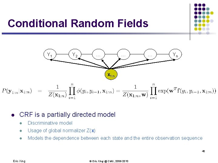
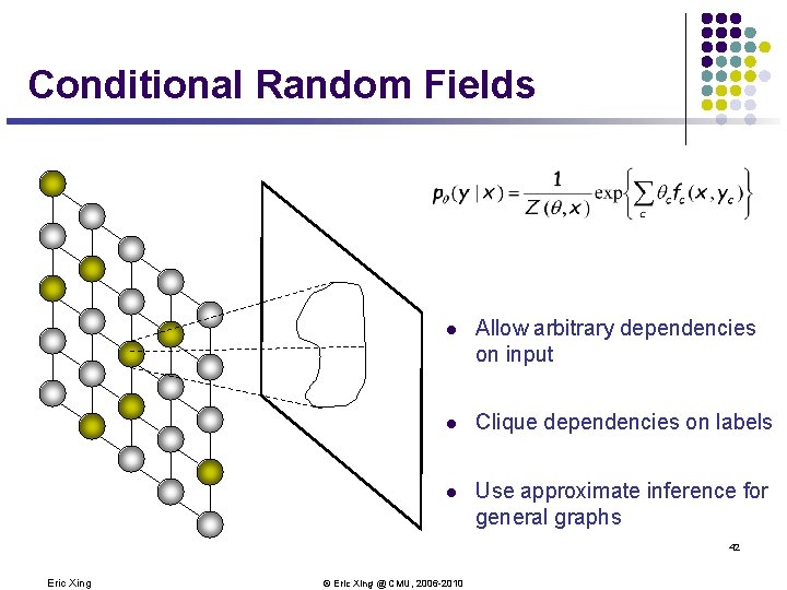
Conditional Random Fields Y 1 Y 2 … … … Yn x 1: n l CRF is a partially directed model l Discriminative model l Usage of global normalizer Z(x) l Models the dependence between each state and the entire observation sequence 40 Eric Xing © Eric Xing @ CMU, 2006 -2010

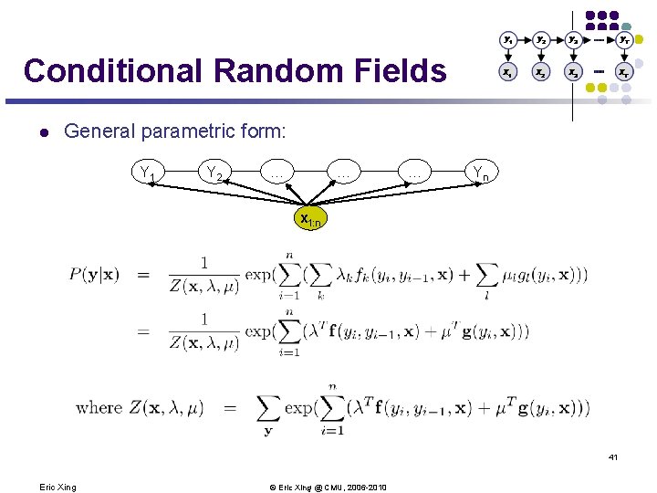
Conditional Random Fields l General parametric form: Y 1 Y 2 … … … Yn x 1: n 41 Eric Xing © Eric Xing @ CMU, 2006 -2010

Conditional Random Fields l Allow arbitrary dependencies on input l Clique dependencies on labels l Use approximate inference for general graphs 42 Eric Xing © Eric Xing @ CMU, 2006 -2010

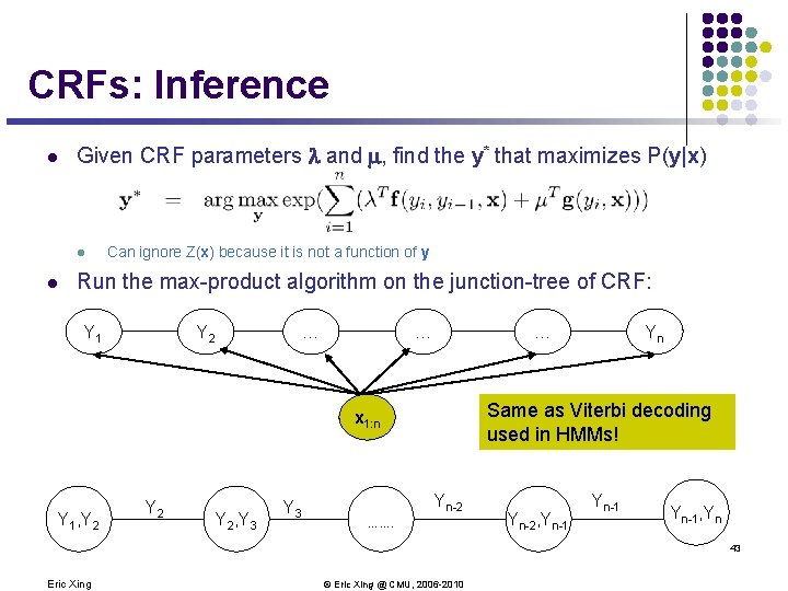
CRFs: Inference l Given CRF parameters and , find the y* that maximizes P(y|x) l l Can ignore Z(x) because it is not a function of y Run the max-product algorithm on the junction-tree of CRF: Y 1 Y 2 … … … Same as Viterbi decoding used in HMMs! x 1: n Y 1, Y 2 Y 2, Y 3 Yn Yn-2 ……. Yn-2, Yn-1, Yn 43 Eric Xing © Eric Xing @ CMU, 2006 -2010

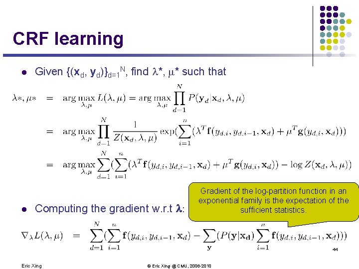
CRF learning l l Given {(xd, yd)}d=1 N, find *, * such that Computing the gradient w. r. t : Gradient of the log-partition function in an exponential family is the expectation of the sufficient statistics. 44 Eric Xing © Eric Xing @ CMU, 2006 -2010

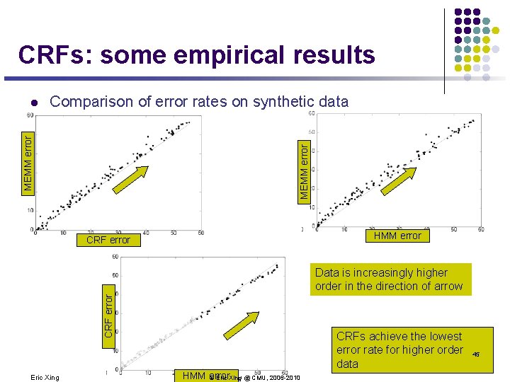
CRFs: some empirical results Comparison of error rates on synthetic data MEMM error l HMM error CRF error Data is increasingly higher order in the direction of arrow Eric Xing CRFs achieve the lowest error rate for higher order data HMM error © Eric Xing @ CMU, 2006 -2010 45

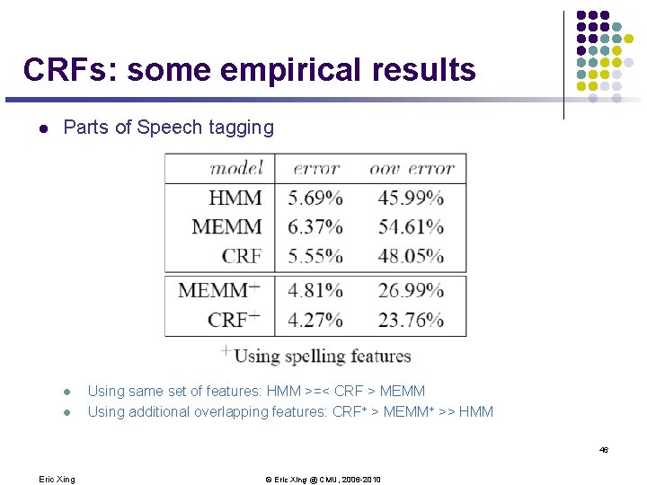
CRFs: some empirical results l Parts of Speech tagging l l Using same set of features: HMM >=< CRF > MEMM Using additional overlapping features: CRF+ > MEMM+ >> HMM 46 Eric Xing © Eric Xing @ CMU, 2006 -2010

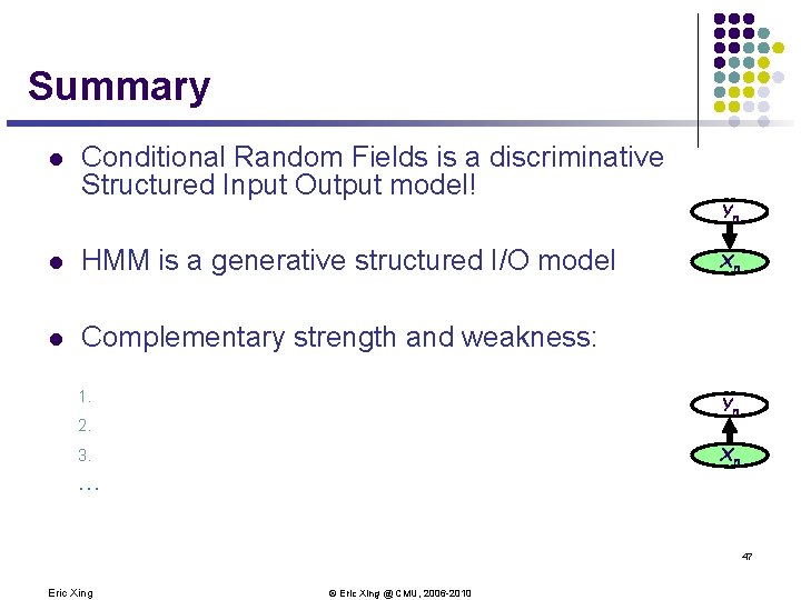
Summary l Conditional Random Fields is a discriminative Structured Input Output model! l HMM is a generative structured I/O model l Complementary strength and weakness: 1. Yn Xn Yn 2. Xn 3. … 47 Eric Xing © Eric Xing @ CMU, 2006 -2010