Machine Learning Robin Burke GAM 376 Outline Terminology

Machine Learning Robin Burke GAM 376

Outline ¢ ¢ Terminology Parameter learning l l ¢ Hill-climbing Simulated annealing Decision learning l l l Decision trees Neural networks Genetic algorithms

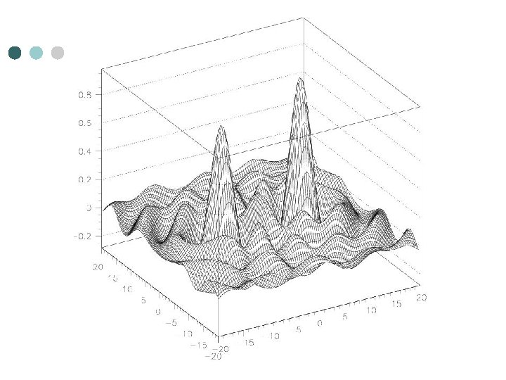
Terminology ¢ On-line learning l ¢ Off-line learning l ¢ a separate learning step that occurs used stored data Over-fitting l l ¢ learning that takes place while the system is operational arises when a learner adapts too completely to off-line data can't cope with novel situations Fitness landscape l l A way to visualize the learning process Fitness = good outcomes n dimensions to adjust behavior which one gets us to the "peak"

Parameter learning ¢ ¢ ¢ A variable or set of variables Different performance at different points in the parameter space Example l Parameters • max. kick velocity • max. running velocity • max. steering force l Performance metric • time of possession

Hill Climbing ¢ ¢ We want to find the best combination of values l cannot simply try them all l there may be many, many possibilities l there may be many dimensions l each test may be expensive Simple idea l pick a point l test its fitness l test neighbors in each dimension • or in some nearby region l l move to the point that is most fit repeat

Step size ¢ How near do I look? step size too small = lots of tests l step size too big = might miss a narrow peak l ¢ Fix l adaptive resolution • at the beginning of the search, large step size • at the end of the search, small step

Local minimum ¢ Can get stuck in a "foothill" l ¢ even if there is a better peak elsewhere Fixes l Momentum • prefer the direction of past movement • sometimes overshooting will carry past a local minimum l Random restart • repeat many times with different random starting points

Simulated annealing ¢ Annealing l l ¢ process of cooling metal slowly creates better crystalline structure Why is this? l l heat is essentially random motion of molecules the lowest-energy state of the system is the most stable • no energy to be gained by changing things l if heat is removed suddenly • the system may be "frozen" in an unstable state

Learning analogy ¢ ¢ Introduce "heat" l randomness in state change l add a random term to fitness assessment l we don't always go "up" the real fitness gradient After k steps of climbing l reduce the temperature l the process converges to regular hill-climbing • when temp = 0 l but the randomness makes sure that more of the parameter space is explored • harder to miss big optima

Decision learning ¢ ¢ ¢ Game AI makes many decisions l when to select which weapon l when to pass, shoot or dribble l when to switch to attack or retreat state We can think of these choices as rule-governed l if a, b, c have particular values, then do x l if a, b, c have other values, then do y Or we can think of them as a divided space l a, b and c are dimensions l x and y are regions of the space • where different behaviors are appropriate

Example ¢ We want to learn l ¢ Then we will know l l ¢ a boundary between the regions for any given parameter combination what decision to make Classification learning

Feedback ¢ Most learning methods are "supervised" l the learning algorithm gets examples • sets of parameters l is told what the right decision is • in each case ¢ The goal is to be able to produce the right classification l for examples not seen originally

Dimensionality ¢ ¢ The more dimensions l the harder the decision boundary is to learn Example l learn how to play Counter-Strike • too many dimensions of input • too many kinds of decisions l learn where to expect an enemy ambush • input = map features • classification simple ¢ Better to learn bits and pieces l than fullscale behavior l not very much like human learning

Decision trees ¢ The idea produce a tree l where each node is a feature value l discriminate your concept l ¢ Learn the decision tree by examining examples l looking for features that divide up the space of examples l

Example

Data class body covering habitat flies? breathes air? 1 m hair land no yes 2 m hair land yes 3 m other water no yes 4 b feathers land yes 5 b feathers land no yes 6 f scales water no no 7 f scales water yes no 8 f other water no no 9 f scales water no yes 10 r scales land no yes

ID 3 Algorithm ¢ Start with an initial node l ¢ ¢ Choose a feature value that splits the examples most nearly in half For each subnode l ¢ (all examples) do this again Continue until all of the examples in the node l have the same class

Information theory ¢ Information as a measurable quantity l ¢ ¢ "a difference that makes a difference" Measured by number of bits needed to send a message Example l l Language A, B, C, D Might need two bits per symbol • ¢ What if you know something about distribution l l l ¢ A=01, B=10, C=00, D=11 C and D are rare (1/8 each) A is common (1/2) B less common (1/4) More efficient coding l l l A=0 B=10 C=110 D=111 1. 75 bits per symbol

Entropy ¢ ¢ What is the smallest number of bits needed to send a message drawn from a given distribution? l depends on the possible symbols l and their frequencies If the symbols all have the same frequency l more information needed to distinguish If some symbols are rare and some high frequency l less information needed This measure is called entropy l in some sense, measures the "disorder" of the distribution

Information gain ¢ The difference between entropy values l ¢ If one distribution has a lower entropy than another l ¢ is called information gain we say it has gained information In ID 3 l l we want each node to eventually have 0 entropy all of the examples agree on the action

Example Health Position Ammo Action 1 Healthy In Cover With Ammo Attack 2 Hurt In Cover With Ammo Attack 3 Healthy In Cover Empty Defend 4 Hurt In Cover Empty Defend 5 Hurt Exposed With Ammo Defend

Entropy ¢ ¢ E = -p. A log 2 p. A – p. D log 2 p. D The entropy of the whole set l ¢ Question l ¢ l l E(healthy) = 1, E(hurt) = 0. 918 E(cover) = 1, E(exposed) = 0. 0 E(ammo) = 0. 918, E(empty) = 0. 0 Information gain l l l ¢ What attribute divides the set into the lowest entropy pieces? Health l ¢ 0. 971 current entropy minus the entropy of each set * the number of examples classified G = E - |T| * ET - |~T|*E~T Example l l l G(health) = 0. 020 G(cover) = 0. 171 G(ammo) = 0. 420

Result Ammo? Yes No Defend Cover? No Defend Yes Attack

Extensions ¢ There are extensions to deal with multiple classes l discrete attributes l continuous attributes l • with some caveats

Neural Networks

Biological inspiration axon dendrites synapses The information transmission happens at the synapses.

Biological inspiration • Tiny voltage spikes travel along the axon of the presynaptic neuron • Trigger the release of neurotransmitter substances at the synapse. • Cause excitation or inhibition in the dendrite of the postsynaptic neuron. • Integration of the signals may produce spikes in the next neuron. • Depends on the strength of the synaptic connection.

Artificial neurons Neurons work by processing information. They receive and provide information in form of voltage spikes. x 1 w 1 x 2 Inputs … xn-1 xn Output y w 2 x 3. . w 3. wn-1 wn The Mc. Cullogh-Pitts model

Artificial neurons The Mc. Cullogh-Pitts model: • spikes are interpreted as spike rates; • synaptic strength are translated as synaptic weights; • excitation means positive product between the incoming spike rate and the corresponding synaptic weight; • inhibition means negative product between the incoming spike rate and the corresponding synaptic weight;

Artificial neurons Nonlinear generalization of the Mc. Cullogh-Pitts neuron: y is the neuron’s output, x is the vector of inputs, and w is the vector of synaptic weights. Examples: sigmoidal neuron Gaussian neuron

Artificial neural networks Inputs Output An artificial neural network is composed of many artificial neurons that are linked together according to a specific network architecture. The objective of the neural network is to transform the inputs into meaningful outputs.

Artificial neural networks Tasks to be solved by artificial neural networks: • controlling the movements of an agent based on selfperception and other information (e. g. , environment information); • deciding the category of situations (e. g. , dangerous or safe) in the game world; • recognizing a pattern of behavior; • predicting what an enemy will do next.

Learning in biological systems • Learning = learning by adaptation • green fruits are sour • yellowish/reddish ones are sweet • adapt picking behavior • Neural level • changing of the synaptic strengths, eliminating some synapses, and building new ones • Form of optimization • Best outcome for least resource usage

Learning principle for artificial neural networks ENERGY MINIMIZATION We need an appropriate definition of energy for artificial neural networks, and having that we can use mathematical optimisation techniques to find how to change the weights of the synaptic connections between neurons. ENERGY = measure of task performance error

Neural network mathematics Inputs Output

MLP neural networks MLP = multi-layer perceptron Perceptron: x yout MLP neural network: x yout

Neural network tasks • control • classification • prediction • approximation These can be reformulated in general as FUNCTION APPROXIMATION tasks. Approximation: given a set of values of a function g(x) build a neural network that approximates the g(x) values for any input x.
, yt=g(xt) +")
Neural network approximation Task specification: Data: set of value pairs: (xt, yt), yt=g(xt) + zt; zt is random measurement noise. Objective: find a neural network that represents the input / output transformation (a function) F(x, W) such that F(x, W) approximates g(x) for every x

Learning to approximate Error measure: Rule for changing the synaptic weights: c is the learning parameter (usually a constant)

Learning with backpropagation A simplification of the learning problem: • calculate first the changes for the synaptic weights of the output neuron; • calculate the changes backward starting from layer p-1, and propagate backward the local error terms. The method is still relatively complicated but it is much simpler than the original optimization problem.

Issues with ANN ¢ ¢ ¢ Often many iterations are needed l 1000 s or even millions Overfitting can be a serious problem No way to diagnose or debug the network l must relearn Designing the network is an art l input and output coding l layering l often learning simply fails Stability vs plasticity l Learning is usually one-shot l Cannot easily restart learning with new data

Genetic Algorithms ¢ ¢ A class of probabilistic optimization algorithms Inspired by the biological evolution process Uses concepts of “Natural Selection” and “Genetic Inheritance” (Darwin 1859) Originally developed by John Holland (1975)
 ¢ ¢ Particularly well suited for hard problems where little is")
GA overview (cont) ¢ ¢ Particularly well suited for hard problems where little is known about the underlying search space Widely-used in business, science, engineering l starting to be used in games and digital cinema

Definition ¢ A genetic algorithm maintains a population of candidate solutions for the problem at hand, and makes it evolve by iteratively applying a set of stochastic operators

Stochastic operators ¢ ¢ ¢ Selection replicates the most successful solutions found in a population at a rate proportional to their relative quality Recombination decomposes two distinct solutions and then randomly mixes their parts to form novel solutions Mutation randomly perturbs a candidate solution

The Metaphor Genetic Algorithm Nature Optimization problem Environment Feasible solutions Individuals living in that environment Individual’s degree of adaptation to its surrounding environment Solutions quality (fitness function)
 Genetic Algorithm A set of feasible solutions Stochastic operators Nature A")
The Metaphor (cont) Genetic Algorithm A set of feasible solutions Stochastic operators Nature A population of organisms (species) Selection, recombination and mutation in nature’s evolutionary process Iteratively applying a set of Evolution of populations to stochastic operators on a set suit their environment of feasible solutions
 The computer model introduces simplifications (relative to the real biological mechanisms),")
The Metaphor (cont) The computer model introduces simplifications (relative to the real biological mechanisms), BUT surprisingly complex and interesting structures have emerged out of evolutionary algorithms

Simple Genetic Algorithm produce an initial population of individuals evaluate the fitness of all individuals while termination condition not met do select fitter individuals for reproduction recombine between individuals mutate individuals evaluate the fitness of the modified individuals generate a new population End while

The Evolutionary Cycle selection parents modification modified offspring initiate & evaluate population evaluated offspring evaluation deleted members discard

A “Population”

Ranking by Fitness:

Mate Selection: Fittest are copied and replaced less-fit

Mate Selection Roulette: Increasing the likelihood but not guaranteeing the fittest reproduction
")
Crossover: Exchanging information through some part of information (representation)

Mutation: Random change of binary digits from 0 to 1 and vice versa (to avoid local minima)

Best Design

The GA Cycle

Example: Karl Sim’s creatures ¢ MIT Media lab

Typical “Chromosome”

Game Applications ¢ Generate behavioral rules l l l ¢ not all the same reasonably effective plausible in the environment Also used in movies l l l battle scenes in "Lord of the Rings" don't want every orc to move the same don't want thousands of extras in costume

Issues ¢ ¢ ¢ Creating the representation is an art l difficult to get right the first time l also tricky to choose the right combination of evolutionary operators Computationally intensive l especially when determining "fitness" is complex l Many, many evolutionary steps required l Very problem-dependent Rarely optimal l often odd artifacts develop and stay • just like real evolution l usually in the region of optimality

Bot Project Due Wednesday 5 pm ¢ Tournament Thursday 11: 45 in Game Lab ¢
- Slides: 64