Machine Learning Paper Reading Series Distances between Data

Machine Learning Paper Reading Series Distances between Data Sets Based on Summary Statistics Nikolaj Tatti, JMLR, 01/2007 Presented by Yuting Qi ECE Dept. Duke Univ. 02/02/2007

Introduction • Goal: – Define a dissimilarity measure, the constrained minimum (CM) distance, between two data sets D 1 and D 2 by comparing summary statistics of datasets. • Requirements: – It should be a metric. – It should consider the statistical nature of data. – It should be evaluated quickly.

The Constrained Minimum (CM) Distance 1/5 • Definition: – Basic notations: • • D: data set, a finite collection of samples in Ω. Ω: finite sample space, |Ω| is the # of elements in Ω. S: feature function, , known or learned. Θ: frequency, , the average values of S over D, S(D) Example: Ω={A, B, C}, D 1=(C, C, C, A), D 2=(C, A, B, A) The only feature of interest is the proportion of C in the data set, then the feature function S is S(D 1)=3/4, S(D 2)=1/4

The Constrained Minimum (CM) Distance 2/5 – Constrained set of distributions: P is the set of all distributions defined on Ω. Calculated from given data sets We estimate statistics from given data set, then examine the distributions that can produce such statistics. – An alternative definition of : If think Ω={1, 2, …, |Ω|}, P is a set of vectors, u, in R|Ω| satisfying non-negative elements and summing to 1. ui=p(i) – Constrained space: Given θ 1 and θ 2, //

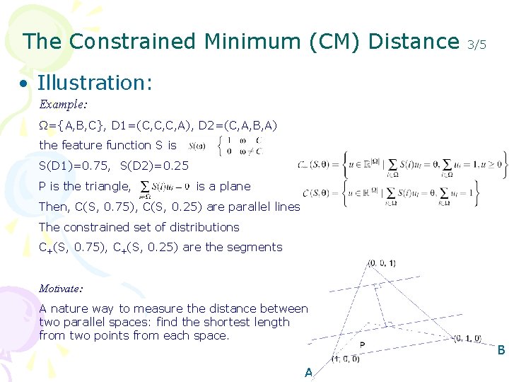
The Constrained Minimum (CM) Distance 3/5 • Illustration: Example: Ω={A, B, C}, D 1=(C, C, C, A), D 2=(C, A, B, A) the feature function S is S(D 1)=0. 75, S(D 2)=0. 25 P is the triangle, is a plane Then, C(S, 0. 75), C(S, 0. 25) are parallel lines The constrained set of distributions C C+(S, 0. 75), C+(S, 0. 25) are the segments Motivate: A nature way to measure the distance between two parallel spaces: find the shortest length from two points from each space. A B

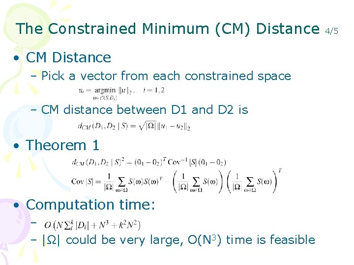
The Constrained Minimum (CM) Distance • CM Distance – Pick a vector from each constrained space – CM distance between D 1 and D 2 is • Theorem 1 • Computation time: – – |Ω| could be very large, O(N 3) time is feasible 4/5

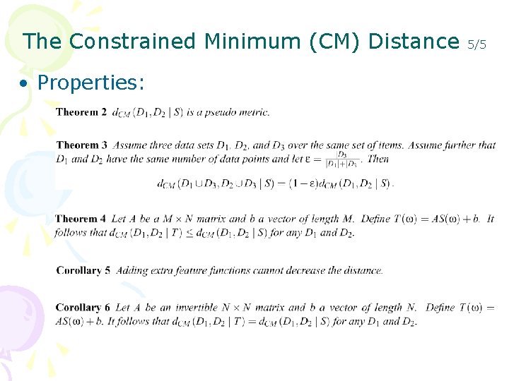
The Constrained Minimum (CM) Distance • Properties: 5/5

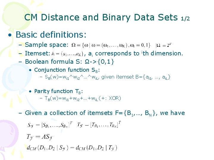
CM Distance and Binary Data Sets 1/2 • Basic definitions: – Sample space: – Itemset: , ai corresponds to ith dimension. – Boolean formula S: Ω->{0, 1} • Conjunction function SB: – SB(w)=wi 1^wi 2^…^wi. L, given itemset B={ai 1, …, ai. L} • Parity function TB: – TB(w)=wi 1+wi 2+…+wi. L (+: XOR) – Given a collection of itemsets F={B 1, …, BN}, we have

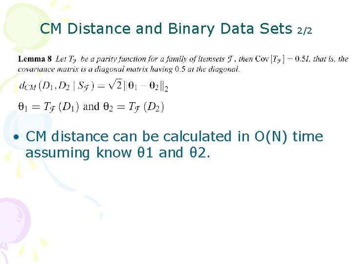
CM Distance and Binary Data Sets 2/2 • CM distance can be calculated in O(N) time assuming know θ 1 and θ 2.

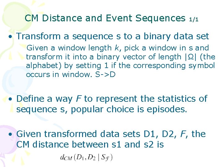
CM Distance and Event Sequences 1/1 • Transform a sequence s to a binary data set Given a window length k, pick a window in s and transform it into a binary vector of length |Ω| (the alphabet) by setting 1 if the corresponding symbol occurs in window. S->D • Define a way F to represent the statistics of sequence s, popular choice is episodes. • Given transformed data sets D 1, D 2, F, the CM distance between s 1 and s 2 is

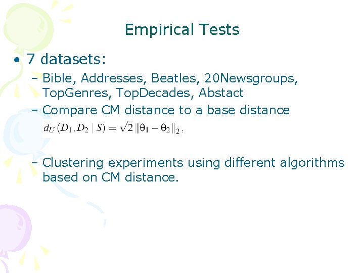
Empirical Tests • 7 datasets: – Bible, Addresses, Beatles, 20 Newsgroups, Top. Genres, Top. Decades, Abstact – Compare CM distance to a base distance – Clustering experiments using different algorithms based on CM distance.

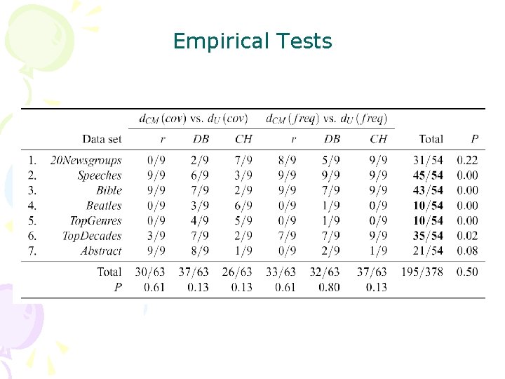
Empirical Tests

Conclusions & Discussion • CM distance has nice statistical properties and can be evaluated efficiently • It takes properly into account the correlation between features • For many types of feature functions, the computation time of CM distance is fast. • The performance of CM distance depends heavily on the data set.