Machine learning overview Computational method to improve performance

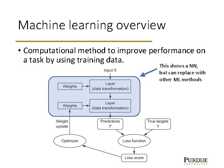
Machine learning overview • Computational method to improve performance on a task by using training data. This shows a NN, but can replace with other ML methods

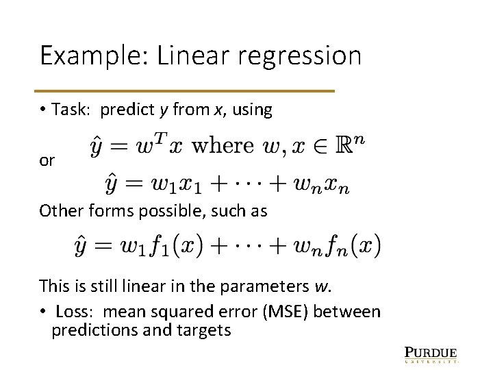
Example: Linear regression • Task: predict y from x, using or Other forms possible, such as This is still linear in the parameters w. • Loss: mean squared error (MSE) between predictions and targets

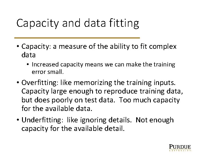
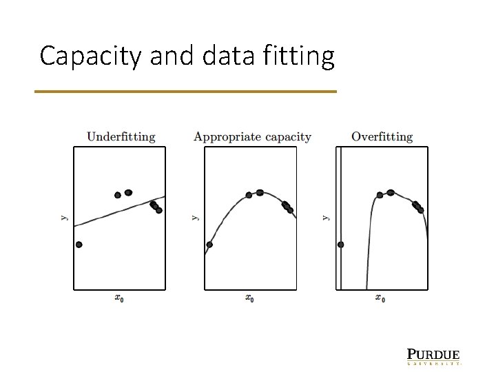
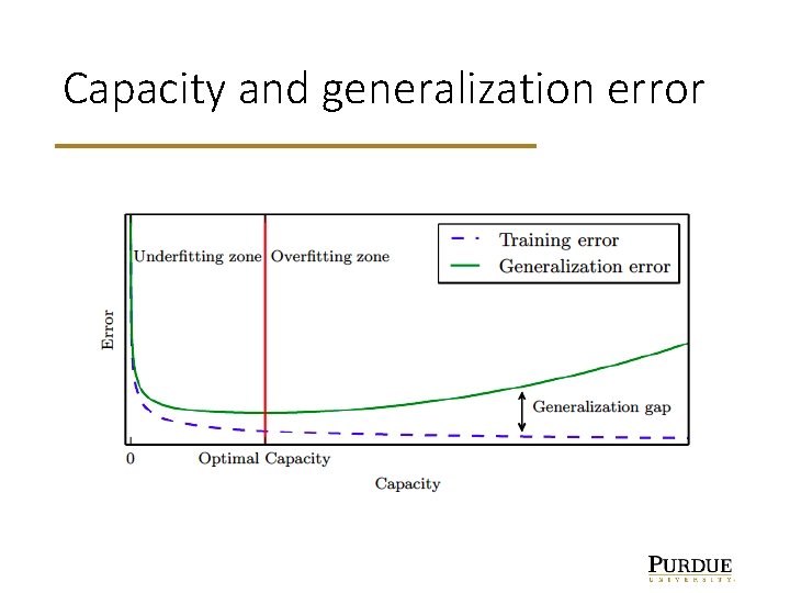
Capacity and data fitting • Capacity: a measure of the ability to fit complex data • Increased capacity means we can make the training error small. • Overfitting: like memorizing the training inputs. Capacity large enough to reproduce training data, but does poorly on test data. Too much capacity for the available data. • Underfitting: like ignoring details. Not enough capacity for the available detail.

Capacity and data fitting

Capacity and generalization error

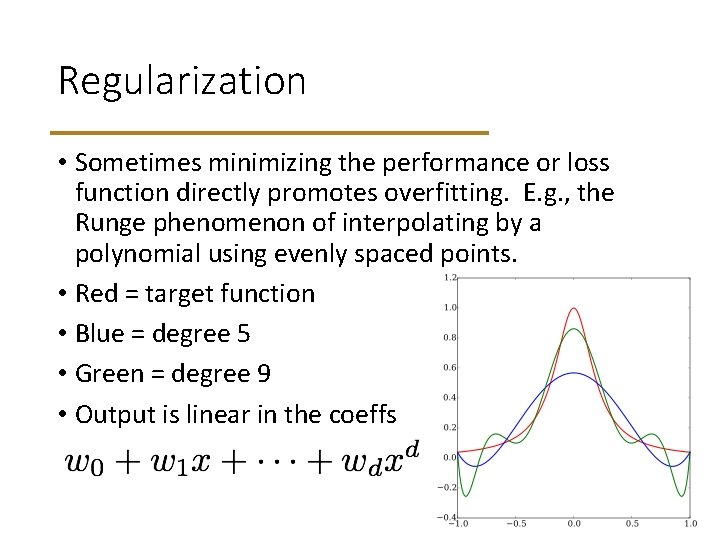
Regularization • Sometimes minimizing the performance or loss function directly promotes overfitting. E. g. , the Runge phenomenon of interpolating by a polynomial using evenly spaced points. • Red = target function • Blue = degree 5 • Green = degree 9 • Output is linear in the coeffs

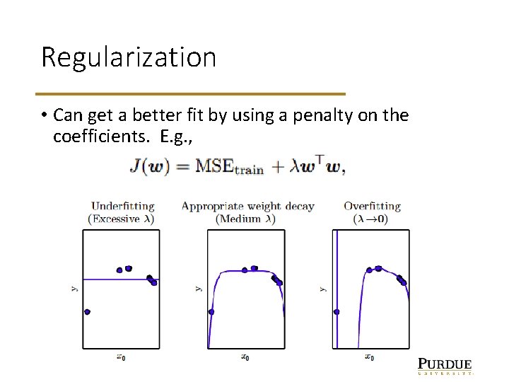
Regularization • Can get a better fit by using a penalty on the coefficients. E. g. ,

Example: Classification • Task: predict one of several classes for a given input. E. g. , • Decide if a movie review is positive or negative. • Identify one of several possible topics for a news piece • Output: A probability distribution on possible outcomes. • Loss: Cross-entropy (a way to compare distributions)

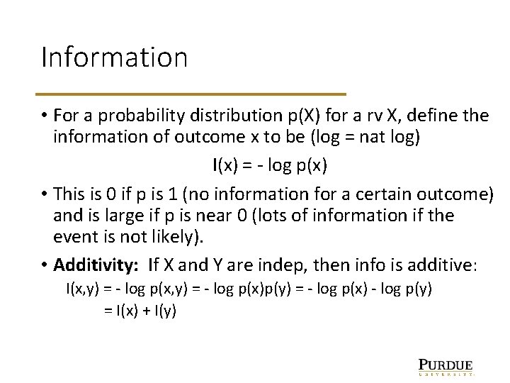
Information • For a probability distribution p(X) for a rv X, define the information of outcome x to be (log = nat log) I(x) = - log p(x) • This is 0 if p is 1 (no information for a certain outcome) and is large if p is near 0 (lots of information if the event is not likely). • Additivity: If X and Y are indep, then info is additive: I(x, y) = - log p(x)p(y) = - log p(x) - log p(y) = I(x) + I(y)

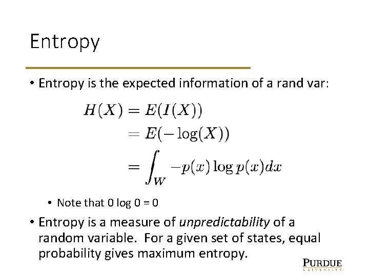
Entropy • Entropy is the expected information of a rand var: • Note that 0 log 0 = 0 • Entropy is a measure of unpredictability of a random variable. For a given set of states, equal probability gives maximum entropy.

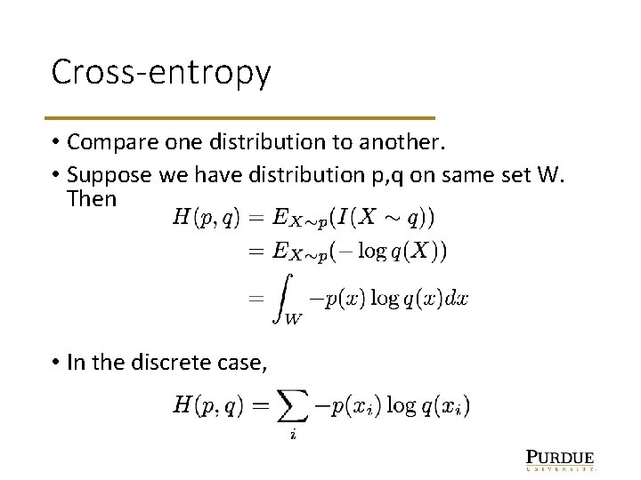
Cross-entropy • Compare one distribution to another. • Suppose we have distribution p, q on same set W. Then • In the discrete case,

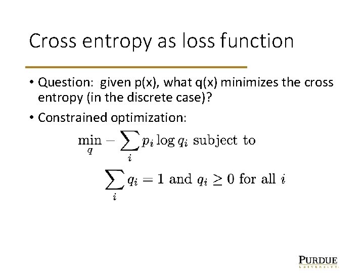
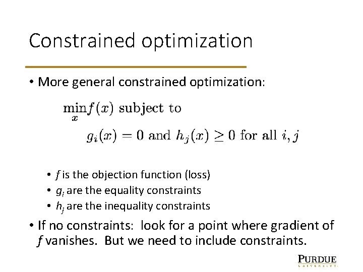
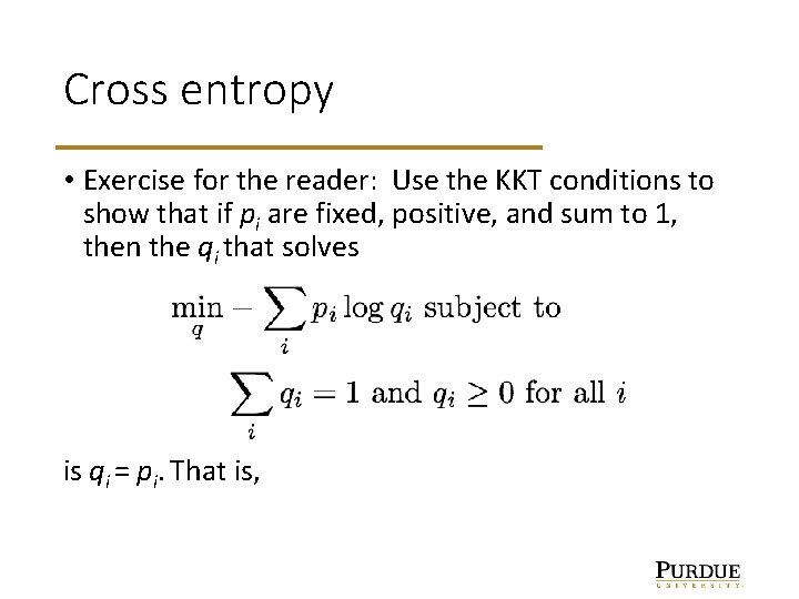
Cross entropy as loss function • Question: given p(x), what q(x) minimizes the cross entropy (in the discrete case)? • Constrained optimization:

Constrained optimization • More general constrained optimization: • f is the objection function (loss) • gi are the equality constraints • hj are the inequality constraints • If no constraints: look for a point where gradient of f vanishes. But we need to include constraints.

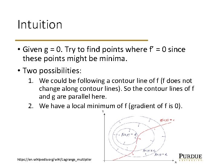
Intuition • Given g = 0. Try to find points where f’ = 0 since these points might be minima. • Two possibilities: 1. We could be following a contour line of f (f does not change along contour lines). So the contour lines of f and g are parallel here. 2. We have a local minimum of f (gradient of f is 0). https: //en. wikipedia. org/wiki/Lagrange_multiplier

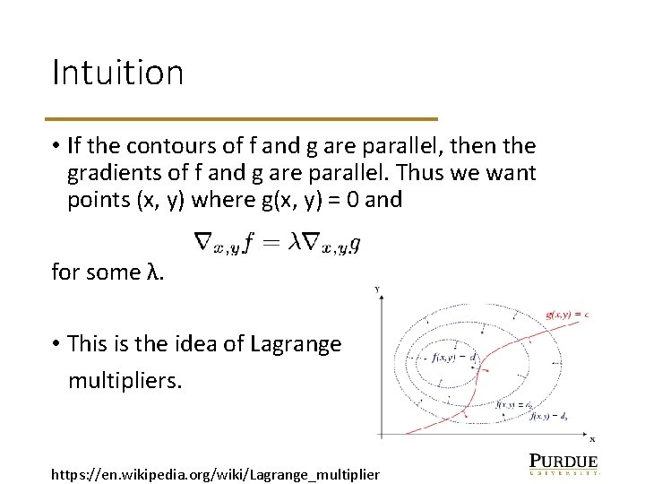
Intuition • If the contours of f and g are parallel, then the gradients of f and g are parallel. Thus we want points (x, y) where g(x, y) = 0 and for some λ. • This is the idea of Lagrange multipliers. https: //en. wikipedia. org/wiki/Lagrange_multiplier

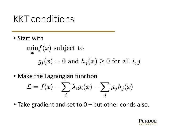
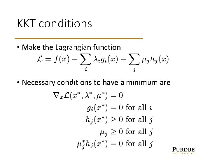
KKT conditions • Start with • Make the Lagrangian function • Take gradient and set to 0 – but other conds also.

KKT conditions • Make the Lagrangian function • Necessary conditions to have a minimum are

Cross entropy • Exercise for the reader: Use the KKT conditions to show that if pi are fixed, positive, and sum to 1, then the qi that solves is qi = pi. That is,

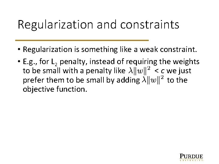
Regularization and constraints • Regularization is something like a weak constraint. • E. g. , for L 2 penalty, instead of requiring the weights to be small with a penalty like < c we just prefer them to be small by adding to the objective function.