Machine Learning Overfitting and Model Selection Eric Xing

Machine Learning Overfitting and Model Selection Eric Xing Lecture 6, August 13, 2010 Reading: © Eric Xing @ CMU, 2006 -2010

Outline l Overfitting l k. NN l Regression l Bias-variance decomposition l Generalization Theory and Structural Risk Minimization l The battle against overfitting: each learning algorithm has some "free knobs" that one can "tune" (i. e. , heck) to make the algorithm generalizes better to test data. But is there a more principled way? l Cross validation l Regularization l Feature selection l Model selection --- Occam's razor l Model averaging © Eric Xing @ CMU, 2006 -2010 2

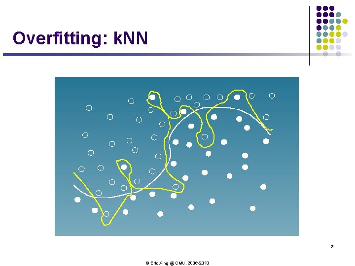
Overfitting: k. NN 3 © Eric Xing @ CMU, 2006 -2010

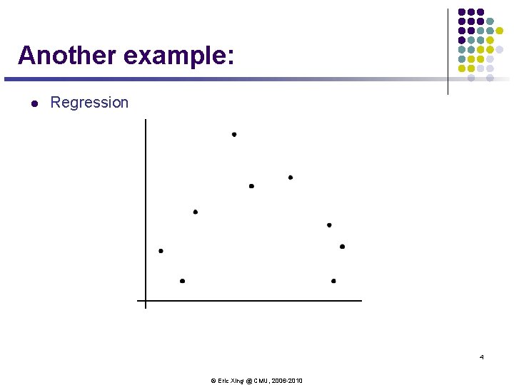
Another example: l Regression 4 © Eric Xing @ CMU, 2006 -2010

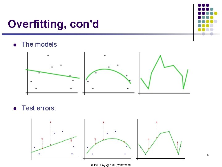
Overfitting, con'd l The models: l Test errors: 5 © Eric Xing @ CMU, 2006 -2010

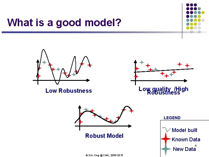
What is a good model? Low Robustness Low quality /High Robustness LEGEND Robust Model built Known Data 6 New Data © Eric Xing @ CMU, 2006 -2010

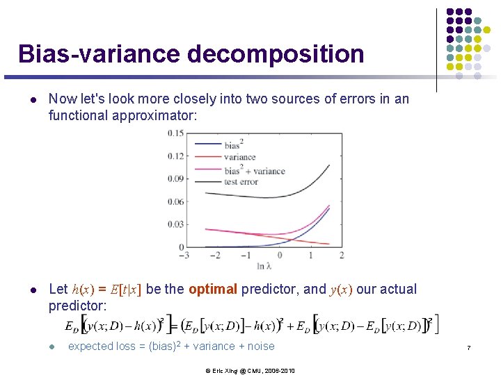
Bias-variance decomposition l Now let's look more closely into two sources of errors in an functional approximator: l Let h(x) = E[t|x] be the optimal predictor, and y(x) our actual predictor: l expected loss = (bias)2 + variance + noise © Eric Xing @ CMU, 2006 -2010 7

Four Pillars for SLT l Consistency (guarantees generalization) l l Model convergence speed (a measure for generalization) l l How does generalization capacity improve when sample size L grows? Generalization capacity control l l Under what conditions will a model be consistent ? How to control in an efficient way model generalization starting with the only given information we have: our sample data? A strategy for good learning algorithms l Is there a strategy that guarantees, measures and controls our learning model generalization capacity ? 8 © Eric Xing @ CMU, 2006 -2010

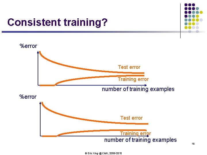
Consistent training? %error Test error Training error number of training examples © Eric Xing @ CMU, 2006 -2010 10

Vapnik main theorem l Q : Under which conditions will a learning model be consistent? l A : A model will be consistent if and only if the function h that defines the model comes from a family of functions H with finite VC dimension d l A finite VC dimension d not only guarantees a generalization capacity (consistency), but to pick h in a family H with finite VC dimension d is the only way to build a model that generalizes. 11 © Eric Xing @ CMU, 2006 -2010

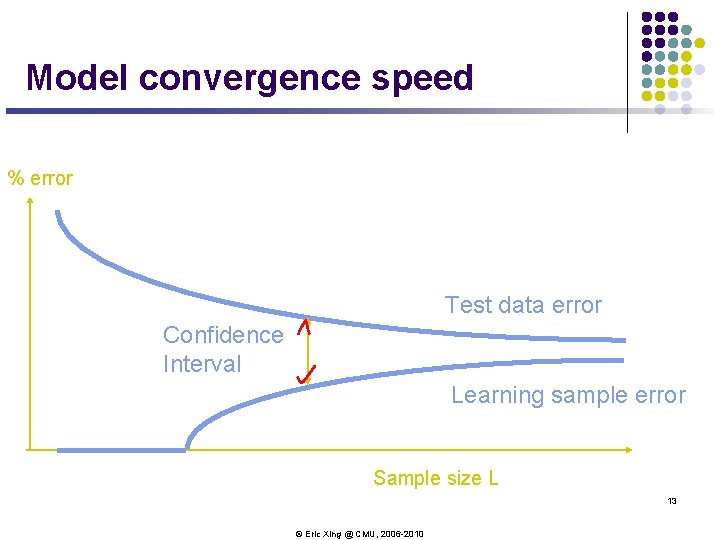
Model convergence speed (generalization capacity) l Q : What is the nature of model error difference between learning data (sample) and test data, for a sample of finite size m? l A : This difference is no greater than a limit that only depends on the ratio between VC dimension d of model functions family H, and sample size m, i. e. , d/m This statement is a new theorem that belongs to Kolmogorov. Smirnov way for results, i. e. , theorems that do not depend on data’s underlying probability law. 12 © Eric Xing @ CMU, 2006 -2010

Model convergence speed % error Test data error Confidence Interval Learning sample error Sample size L 13 © Eric Xing @ CMU, 2006 -2010

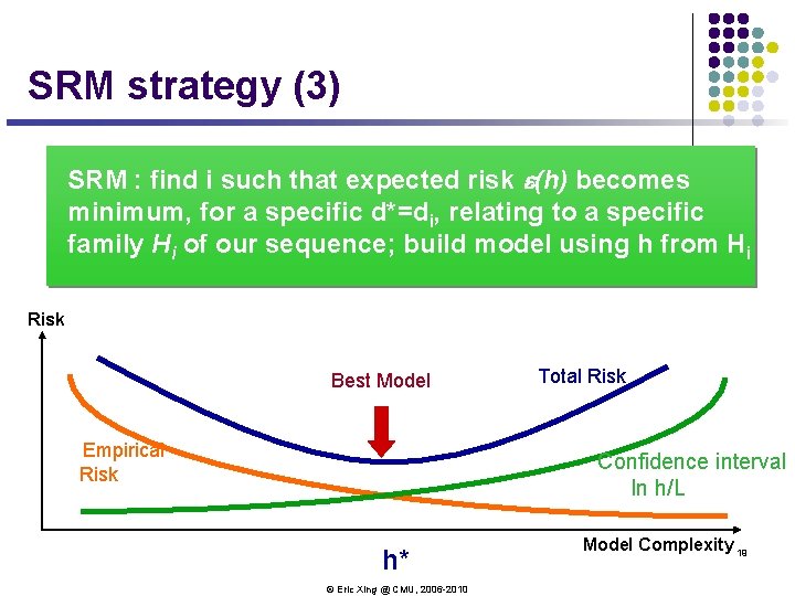
How to control model generalization capacity Risk Expectation = Empirical Risk + Confidence Interval l To minimize Empirical Risk alone will not always give a good generalization capacity: one will want to minimize the sum of Empirical Risk and Confidence Interval l What is important is not the numerical value of the Vapnik limit, most often too large to be of any practical use, it is the fact that this limit is a non decreasing function of model family function “richness” 14 © Eric Xing @ CMU, 2006 -2010

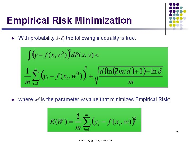
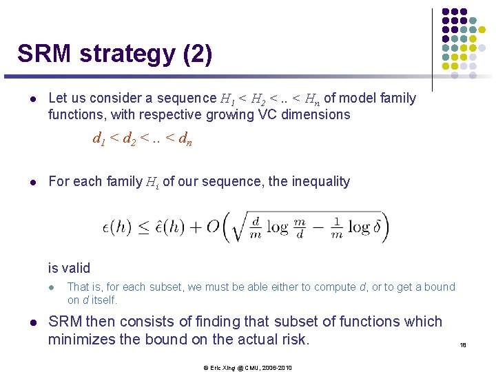
Empirical Risk Minimization l With probability 1 -d, the following inequality is true: l where w 0 is the parameter w value that minimizes Empirical Risk: 15 © Eric Xing @ CMU, 2006 -2010

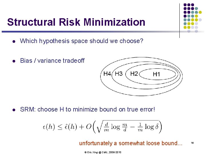
Structural Risk Minimization l Which hypothesis space should we choose? l Bias / variance tradeoff l SRM: choose H to minimize bound on true error! unfortunately a somewhat loose bound. . . © Eric Xing @ CMU, 2006 -2010 16

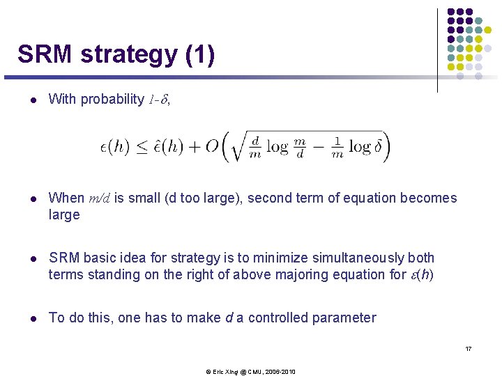
SRM strategy (1) l With probability 1 -d, l When m/d is small (d too large), second term of equation becomes large l SRM basic idea for strategy is to minimize simultaneously both terms standing on the right of above majoring equation for e(h) l To do this, one has to make d a controlled parameter 17 © Eric Xing @ CMU, 2006 -2010

SRM strategy (2) l Let us consider a sequence H 1 < H 2 <. . < Hn of model family functions, with respective growing VC dimensions d 1 < d 2 <. . < dn l For each family Hi of our sequence, the inequality is valid l l That is, for each subset, we must be able either to compute d, or to get a bound on d itself. SRM then consists of finding that subset of functions which minimizes the bound on the actual risk. © Eric Xing @ CMU, 2006 -2010 18

SRM strategy (3) SRM : find i such that expected risk e(h) becomes minimum, for a specific d*=di, relating to a specific family Hi of our sequence; build model using h from Hi Risk Best Model Empirical Risk Total Risk Confidence interval In h/L h* © Eric Xing @ CMU, 2006 -2010 Model Complexity 19

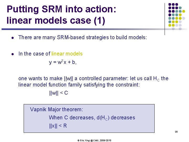
Putting SRM into action: linear models case (1) l There are many SRM-based strategies to build models: l In the case of linear models y = w. Tx + b, one wants to make ||w|| a controlled parameter: let us call HC the linear model function family satisfying the constraint: ||w|| < C Vapnik Major theorem: When C decreases, d(HC) decreases ||x|| < R 20 © Eric Xing @ CMU, 2006 -2010

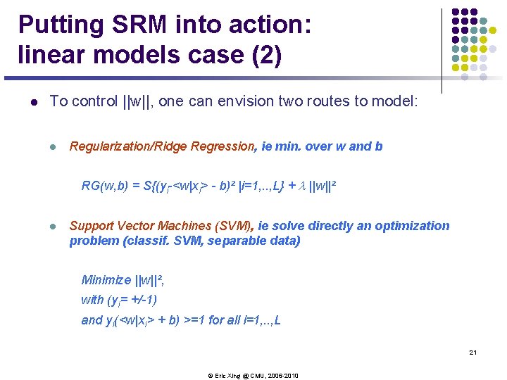
Putting SRM into action: linear models case (2) l To control ||w||, one can envision two routes to model: l Regularization/Ridge Regression, ie min. over w and b RG(w, b) = S{(yi-<w|xi> - b)² |i=1, . . , L} + l ||w||² l Support Vector Machines (SVM), ie solve directly an optimization problem (classif. SVM, separable data) Minimize ||w||², with (yi= +/-1) and yi(<w|xi> + b) >=1 for all i=1, . . , L 21 © Eric Xing @ CMU, 2006 -2010

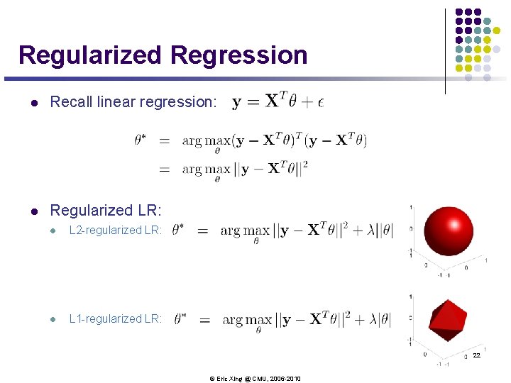
Regularized Regression l Recall linear regression: l Regularized LR: l L 2 -regularized LR: l L 1 -regularized LR: 22 © Eric Xing @ CMU, 2006 -2010

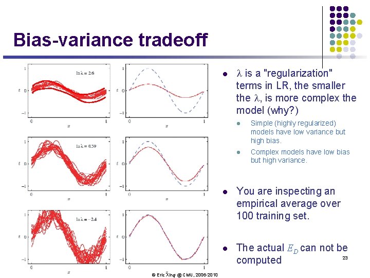
Bias-variance tradeoff l © Eric Xing @ CMU, 2006 -2010 l is a "regularization" terms in LR, the smaller the l, is more complex the model (why? ) l Simple (highly regularized) models have low variance but high bias. l Complex models have low bias but high variance. l You are inspecting an empirical average over 100 training set. l The actual ED can not be 23 computed

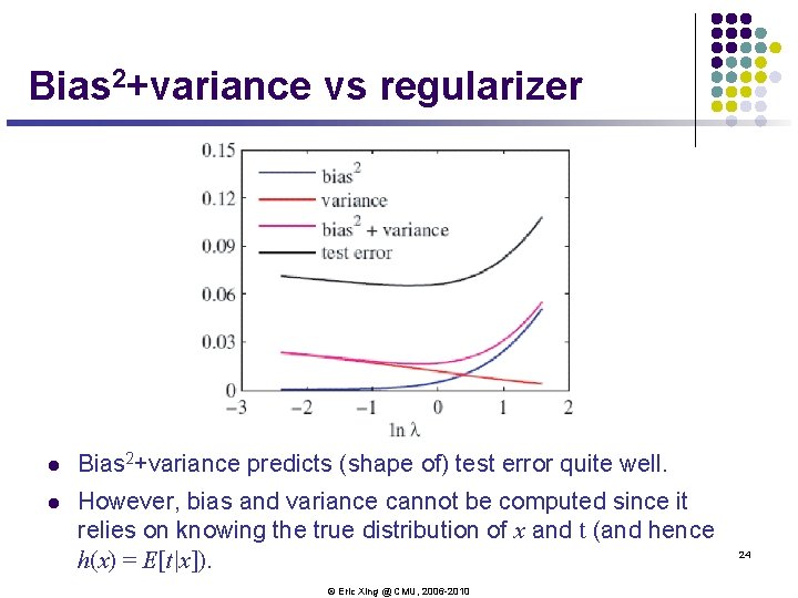
Bias 2+variance vs regularizer l Bias 2+variance predicts (shape of) test error quite well. l However, bias and variance cannot be computed since it relies on knowing the true distribution of x and t (and hence h(x) = E[t|x]). © Eric Xing @ CMU, 2006 -2010 24

The battle against overfitting 25 © Eric Xing @ CMU, 2006 -2010

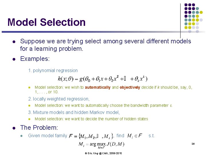
Model Selection l Suppose we are trying select among several different models for a learning problem. l Examples: 1. polynomial regression l Model selection: we wish to automatically and objectively decide if k should be, say, 0, 1, . . . , or 10. 2. locally weighted regression, l Model selection: we want to automatically choose the bandwidth parameter t. 3. Mixture models and hidden Markov model, l l Model selection: we want to decide the number of hidden states The Problem: l Given model family , find s. t. 26 © Eric Xing @ CMU, 2006 -2010

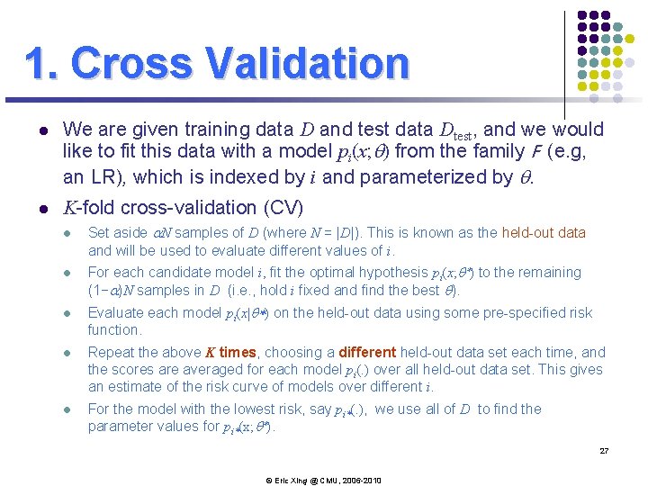
1. Cross Validation l We are given training data D and test data Dtest, and we would like to fit this data with a model pi(x; q) from the family F (e. g, an LR), which is indexed by i and parameterized by q. l K-fold cross-validation (CV) l l l Set aside a. N samples of D (where N = |D|). This is known as the held-out data and will be used to evaluate different values of i. For each candidate model i, fit the optimal hypothesis pi(x; q*) to the remaining (1−a)N samples in D (i. e. , hold i fixed and find the best q). Evaluate each model pi(x|q*) on the held-out data using some pre-specified risk function. l Repeat the above K times, choosing a different held-out data set each time, and the scores are averaged for each model pi(. ) over all held-out data set. This gives an estimate of the risk curve of models over different i. l For the model with the lowest risk, say pi*(. ), we use all of D to find the parameter values for pi*(x; q*). 27 © Eric Xing @ CMU, 2006 -2010

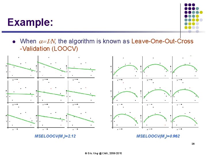
Example: l When a=1/N, the algorithm is known as Leave-One-Out-Cross -Validation (LOOCV) MSELOOCV(M 1)=2. 12 MSELOOCV(M 2)=0. 962 28 © Eric Xing @ CMU, 2006 -2010

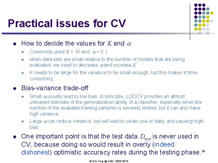
Practical issues for CV l How to decide the values for K and a l l l when data sets are small relative to the number of models that are being evaluated, we need to decrease a and increase K l K needs to be large for the variance to be small enough, but this makes it timeconsuming. Bias-variance trade-off l l l Commonly used K = 10 and a = 0. 1. Small a usually lead to low bias. In principle, LOOCV provides an almost unbiased estimate of the generalization ability of a classifier, especially when the number of the available training samples is severely limited; but it can also have high variance. Large a can reduce variance, but will lead to under-use of data, and causing highbias. One important point is that the test data Dtest is never used in CV, because doing so would result in overly (indeed dishonest) optimistic accuracy rates during the testing phase. 29 © Eric Xing @ CMU, 2006 -2010

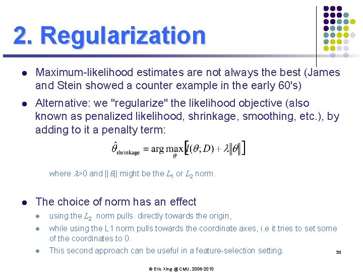
2. Regularization l Maximum-likelihood estimates are not always the best (James and Stein showed a counter example in the early 60's) l Alternative: we "regularize" the likelihood objective (also known as penalized likelihood, shrinkage, smoothing, etc. ), by adding to it a penalty term: where l>0 and ||q|| might be the L 1 or L 2 norm. l The choice of norm has an effect l using the L 2 norm pulls directly towards the origin, l while using the L 1 norm pulls towards the coordinate axes, i. e it tries to set some of the coordinates to 0. l This second approach can be useful in a feature-selection setting. © Eric Xing @ CMU, 2006 -2010 30

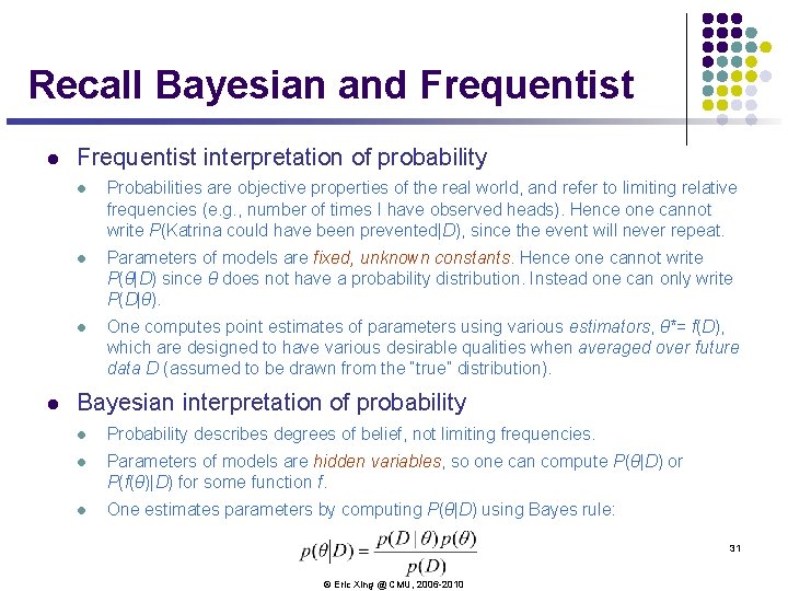
Recall Bayesian and Frequentist l l Frequentist interpretation of probability l Probabilities are objective properties of the real world, and refer to limiting relative frequencies (e. g. , number of times I have observed heads). Hence one cannot write P(Katrina could have been prevented|D), since the event will never repeat. l Parameters of models are fixed, unknown constants. Hence one cannot write P(θ|D) since θ does not have a probability distribution. Instead one can only write P(D|θ). l One computes point estimates of parameters using various estimators, θ*= f(D), which are designed to have various desirable qualities when averaged over future data D (assumed to be drawn from the “true” distribution). Bayesian interpretation of probability l Probability describes degrees of belief, not limiting frequencies. l Parameters of models are hidden variables, so one can compute P(θ|D) or P(f(θ)|D) for some function f. l One estimates parameters by computing P(θ|D) using Bayes rule: 31 © Eric Xing @ CMU, 2006 -2010

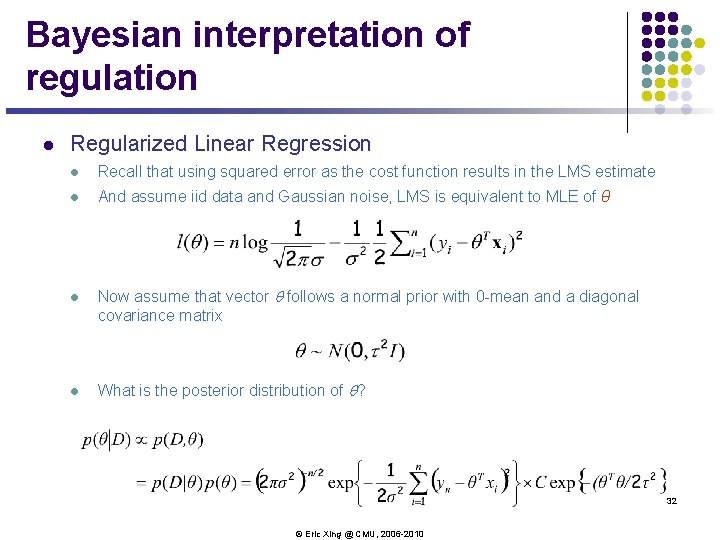
Bayesian interpretation of regulation l Regularized Linear Regression l Recall that using squared error as the cost function results in the LMS estimate l And assume iid data and Gaussian noise, LMS is equivalent to MLE of θ l l Now assume that vector q follows a normal prior with 0 -mean and a diagonal covariance matrix What is the posterior distribution of q? 32 © Eric Xing @ CMU, 2006 -2010

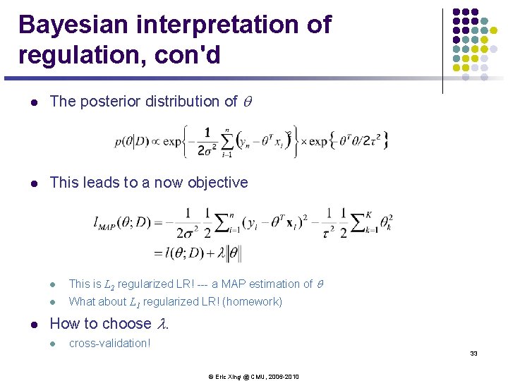
Bayesian interpretation of regulation, con'd l The posterior distribution of q l This leads to a now objective l l This is L 2 regularized LR! --- a MAP estimation of q l What about L 1 regularized LR! (homework) How to choose l. l cross-validation! 33 © Eric Xing @ CMU, 2006 -2010

3. Feature Selection l Imagine that you have a supervised learning problem where the number of features d is very large (perhaps d >>#samples), but you suspect that there is only a small number of features that are "relevant" to the learning task. l VC-theory can tell you that this scenario is likely to lead to high generalization error – the learned model will potentially overfit unless the training set is fairly large. l So lets get rid of useless parameters! 34 © Eric Xing @ CMU, 2006 -2010

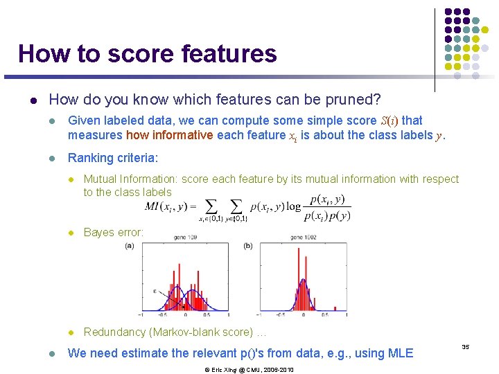
How to score features l How do you know which features can be pruned? l Given labeled data, we can compute some simple score S(i) that measures how informative each feature xi is about the class labels y. l Ranking criteria: l l Mutual Information: score each feature by its mutual information with respect to the class labels l Bayes error: l Redundancy (Markov-blank score) … We need estimate the relevant p()'s from data, e. g. , using MLE © Eric Xing @ CMU, 2006 -2010 35

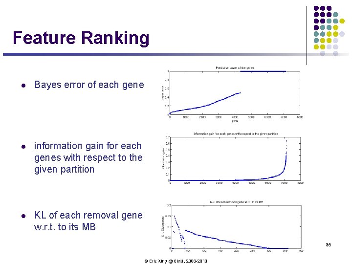
Feature Ranking l Bayes error of each gene l information gain for each genes with respect to the given partition l KL of each removal gene w. r. t. to its MB 36 © Eric Xing @ CMU, 2006 -2010

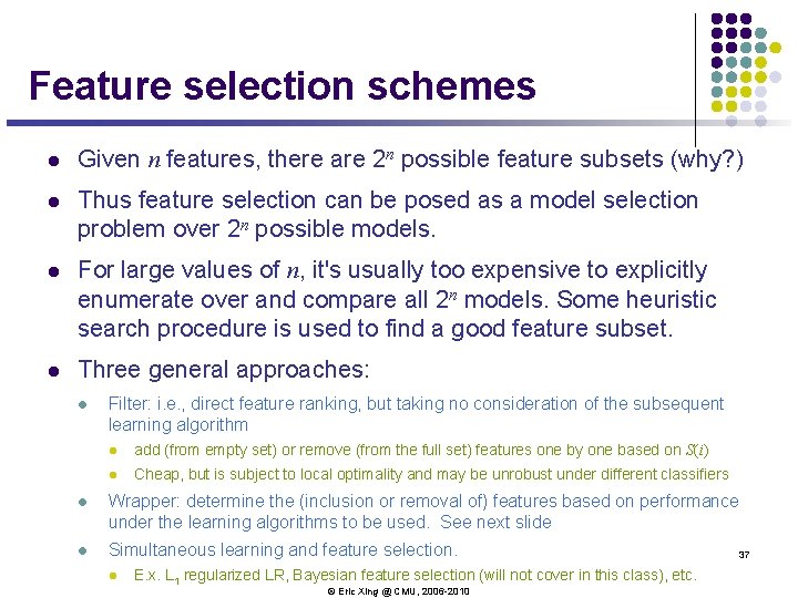
Feature selection schemes l Given n features, there are 2 n possible feature subsets (why? ) l Thus feature selection can be posed as a model selection problem over 2 n possible models. l For large values of n, it's usually too expensive to explicitly enumerate over and compare all 2 n models. Some heuristic search procedure is used to find a good feature subset. l Three general approaches: l Filter: i. e. , direct feature ranking, but taking no consideration of the subsequent learning algorithm l add (from empty set) or remove (from the full set) features one by one based on S(i) l Cheap, but is subject to local optimality and may be unrobust under different classifiers l Wrapper: determine the (inclusion or removal of) features based on performance under the learning algorithms to be used. See next slide l Simultaneous learning and feature selection. l E. x. L 1 regularized LR, Bayesian feature selection (will not cover in this class), etc. © Eric Xing @ CMU, 2006 -2010 37

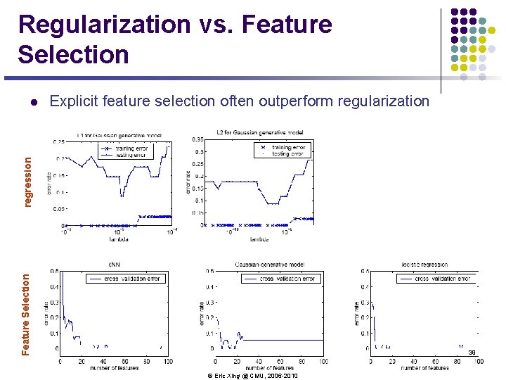
Case study l [Xing et al, 2001] The case: l 7130 genes from a microarray dataset l 72 samples l 47 type I Leukemias (called ALL) and 25 type II Leukemias (called AML) l Three classifier: l k. NN l Gaussian classifier l Logistic regression 38 © Eric Xing @ CMU, 2006 -2010

Regularization vs. Feature Selection Explicit feature selection often outperform regularization Feature Selection regression l 39 © Eric Xing @ CMU, 2006 -2010

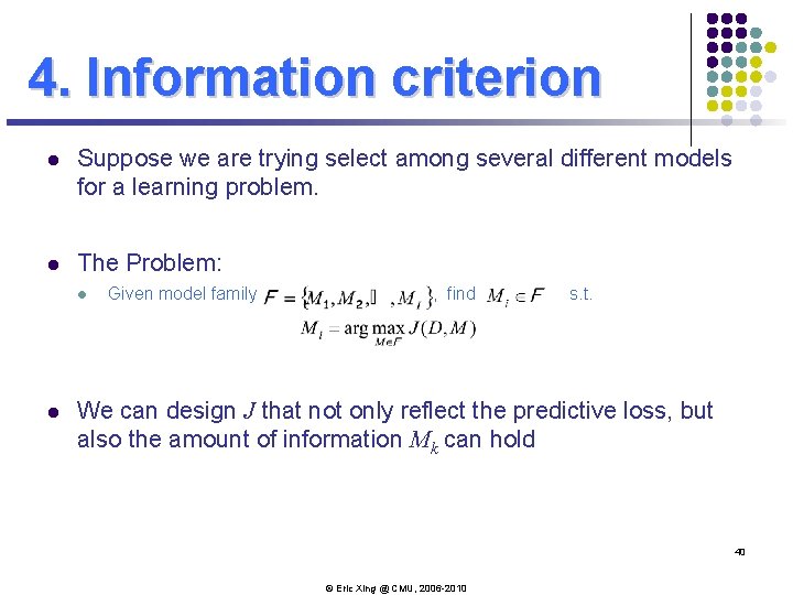
4. Information criterion l Suppose we are trying select among several different models for a learning problem. l The Problem: l l Given model family , find s. t. We can design J that not only reflect the predictive loss, but also the amount of information Mk can hold 40 © Eric Xing @ CMU, 2006 -2010

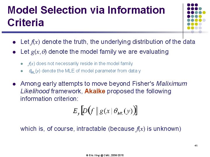
Model Selection via Information Criteria l Let f(x) denote the truth, the underlying distribution of the data l Let g(x, q) denote the model family we are evaluating l l f(x) does not necessarily reside in the model family l q. ML(y) denote the MLE of model parameter from data y Among early attempts to move beyond Fisher's Maliximum Likelihood framework, Akaike proposed the following information criterion: which is, of course, intractable (because f(x) is unknown) 41 © Eric Xing @ CMU, 2006 -2010

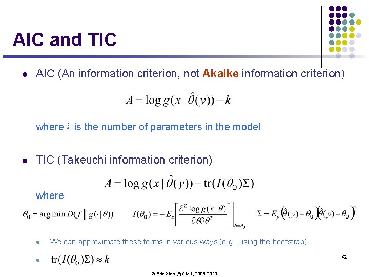
AIC and TIC l AIC (An information criterion, not Akaike information criterion) where k is the number of parameters in the model l TIC (Takeuchi information criterion) where l We can approximate these terms in various ways (e. g. , using the bootstrap) 42 l © Eric Xing @ CMU, 2006 -2010

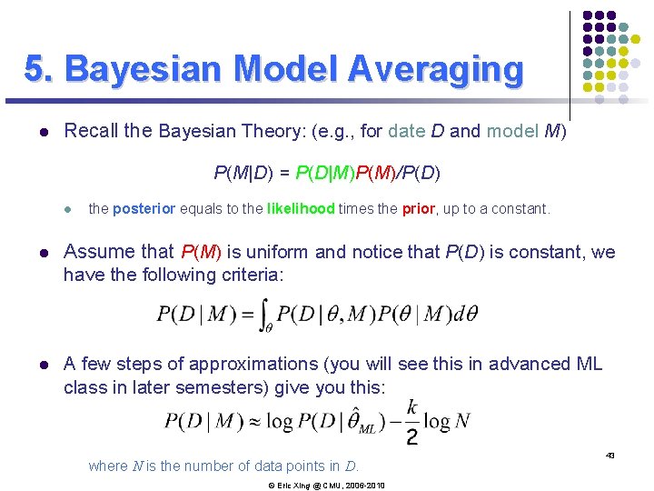
5. Bayesian Model Averaging l Recall the Bayesian Theory: (e. g. , for date D and model M) P(M|D) = P(D|M)P(M)/P(D) l the posterior equals to the likelihood times the prior, up to a constant. l Assume that P(M) is uniform and notice that P(D) is constant, we have the following criteria: l A few steps of approximations (you will see this in advanced ML class in later semesters) give you this: where N is the number of data points in D. © Eric Xing @ CMU, 2006 -2010 43

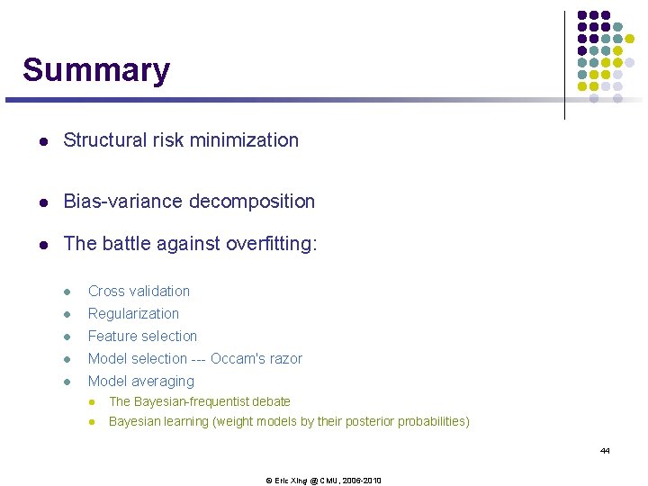
Summary l Structural risk minimization l Bias-variance decomposition l The battle against overfitting: l Cross validation l Regularization l Feature selection l Model selection --- Occam's razor l Model averaging l The Bayesian-frequentist debate l Bayesian learning (weight models by their posterior probabilities) 44 © Eric Xing @ CMU, 2006 -2010