Machine Learning Neural Networks Learning Theory v v

Machine Learning Neural Networks

Learning Theory v v Theorems that characterize classes of learning problems or specific algorithms in terms of computational complexity or sample complexity, i. e. the number of training examples necessary or sufficient to learn hypotheses of a given accuracy. Complexity of a learning problem depends on: – Size or expressiveness of the hypothesis space. – Accuracy to which target concept must be approximated. – Probability with which the learner must produce a successful hypothesis. – Manner in which training examples are presented, e. g. randomly or by query to an oracle. 2

Types of Results v v v Learning in the limit: Is the learner guaranteed to converge to the correct hypothesis in the limit as the number of training examples increases indefinitely? Sample Complexity: How many training examples are needed for a learner to construct (with high probability) a highly accurate concept? Computational Complexity: How much computational resources (time and space) are needed for a learner to construct (with high probability) a highly accurate concept? – High sample complexity implies high computational complexity, since learner at least needs to read the input data. v Mistake Bound: Learning incrementally, how many training examples will the learner misclassify before 3 concept. constructing a highly accurate

Cannot Learn Exact Concepts from Limited Data, Only Approximations Positive Negative Learner Classifier Positive Negative 4

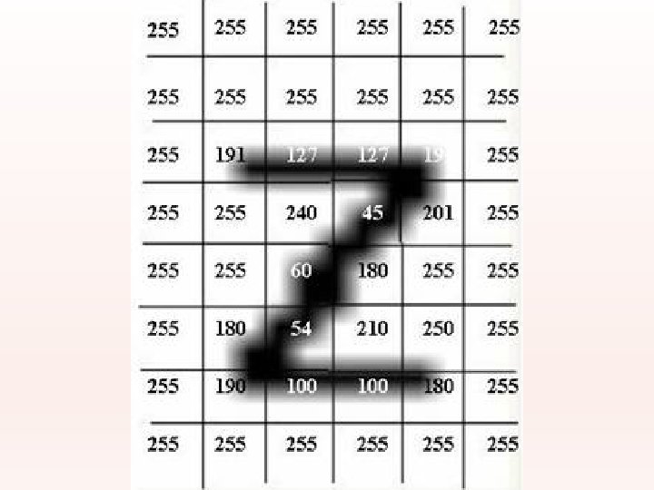
The machine learning framework v Apply a prediction function to a feature representation of the image to get the desired output: f( f( f( ) = “apple” ) = “tomato” ) = “cow”

The machine learning framework y = f(x) output v v prediction function Image feature Training: given a training set of labeled examples {(x 1, y 1), …, (x. N, y. N)}, estimate the prediction function f by minimizing the prediction error on the training set Testing: apply f to a never before seen test example x and output the predicted value y = f(x)

Classification Steps Training Labels Training Images Image Features Training Learned model Prediction Testing Image Features Test Image

Classifiers: Nearest neighbor Training examples from class 1 Test example Training examples from class 2 f(x) = label of the training example nearest to x v v All we need is a distance function for our inputs No training required!

Classifiers: Linear v Find a linear function to separate the classes: f(x) = sgn(w x + b)

Many classifiers to choose from v v v v v SVM Neural networks Naïve Bayesian network Logistic regression Randomized Forests Boosted Decision Trees K-nearest neighbor RBMs Etc. Which is the best one?

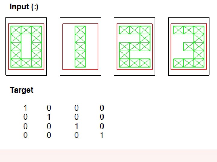
Recognition task and supervision v Images in the training set must be annotated with the “correct answer” that the model is expected to produce Contains a motorbike

Generalization Training set (labels known) v Test set (labels unknown) How well does a learned model generalize from the data it was trained on to a new test set?

Classification Assign input vector to one of two or more classes v Any decision rule divides input space into decision regions separated by decision boundaries v Slide credit: L. Lazebnik

Classifiers: Linear SVM x x o x o o x x x o x 2 x 1 • Find a linear function to separate the classes: f(x) = sgn(w x + b)

Neural Networks v Artificial Neural Network is based on the biological nervous system as Brain v It is composed of interconnected computing units called neurons v ANN like human, learn by examples

Why Artificial Neural Networks? There are two basic reasons why we are interested in building artificial neural networks (ANNs): v Technical viewpoint: Some problems such as character recognition or the prediction of future states of a system require massively parallel and adaptive processing. v Biological viewpoint: ANNs can be used to replicate and simulate components of the human (or animal) brain, thereby giving us insight into natural information processing. 19

Science: Model how biological neural systems, like human brain, work? v How do we see? v How is information stored in/retrieved from memory? v How do you learn to not to touch fire? v How do your eyes adapt to the amount of light in the environment? v Related fields: Neuroscience, Computational Neuroscience, Psychology, Psychophysiology, Cognitive Science, Medicine, Math, Physics. 20

Brief History Old Ages: v Association (William James; 1890) v Mc. Culloch-Pitts Neuron (1943, 1947) v Perceptrons (Rosenblatt; 1958, 1962) v Adaline/LMS (Widrow and Hoff; 1960) v Perceptrons book (Minsky and Papert; 1969) Dark Ages: v Self-organization in visual cortex (von der Malsburg; 1973) v Backpropagation (Werbos, 1974) v Foundations of Adaptive Resonance Theory (Grossberg; 1976) v Neural Theory of Association (Amari; 1977) 21

History Modern Ages: v Adaptive Resonance Theory (Grossberg; 1980) v Hopfield model (Hopfield; 1982, 1984) v Self-organizing maps (Kohonen; 1982) v Reinforcement learning (Sutton and Barto; 1983) v Simulated Annealing (Kirkpatrick et al. ; 1983) v Boltzmann machines (Ackley, Hinton, Terrence; 1985) v Backpropagation (Rumelhart, Hinton, Williams; 1986) v ART-networks (Carpenter, Grossberg; 1992) v Support Vector Machines 22

Hebb’s Learning Law v • • • In 1949, Donald Hebb formulated William James’ principle of association into a mathematical form. If the activation of the neurons, y 1 and y 2 , are both on (+1) then the weight between the two neurons grow. (Off: 0) Else the weight between remains the same. However, when bipolar activation {-1, +1} scheme is used, then the weights can also decrease when the activation of two neurons does not match. 23

Biological Neurons v v v Human brain = tens of thousands of neurons Each neuron is connected to thousands other neurons A neuron is made of: – The soma: body of the neuron – Dendrites: filaments that provide input to the neuron – The axon: sends an output signal – Synapses: connection with other neurons – releases certain quantities of chemicals called neurotransmitters to other neurons 24

Modeling of Brain Functions 25

The biological neuron v v The pulses generated by the neuron travels along the axon as an electrical wave. Once these pulses reach the synapses at the end of the axon open up chemical vesicles exciting the other neuron. 26

How do NNs and ANNs work? v Information is transmitted as a series of electric impulses, so-called spikes. v The frequency and phase of these spikes encodes the information. v In biological systems, one neuron can be connected to as many as 10, 000 other neurons. v Usually, a neuron receives its information from other neurons in a confined area 27

Computers vs. Neural Networks “Standard” Computers Neural Networks one CPU highly parallel processing fast processing units slow processing reliable units unreliable units static infrastructure dynamic 28

Neural Network

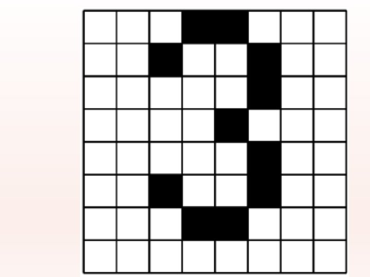
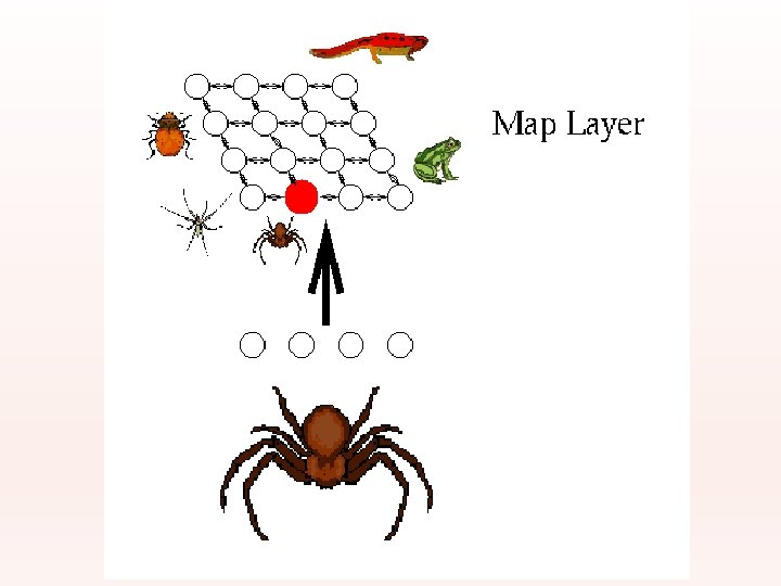
Neural Network Application • Pattern recognition can be implemented using NN • The figure can be T or H character, the network should identify each class of T or H.

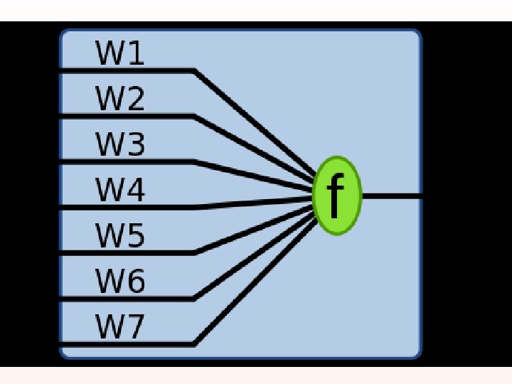
Simple Neuron X 1 Inputs X 2 Output Xn b

An Artificial Neuron synapses neuron i x 1 x 2 Wi, 1 Wi, 2 … Wi, n … xn net input signal output xi

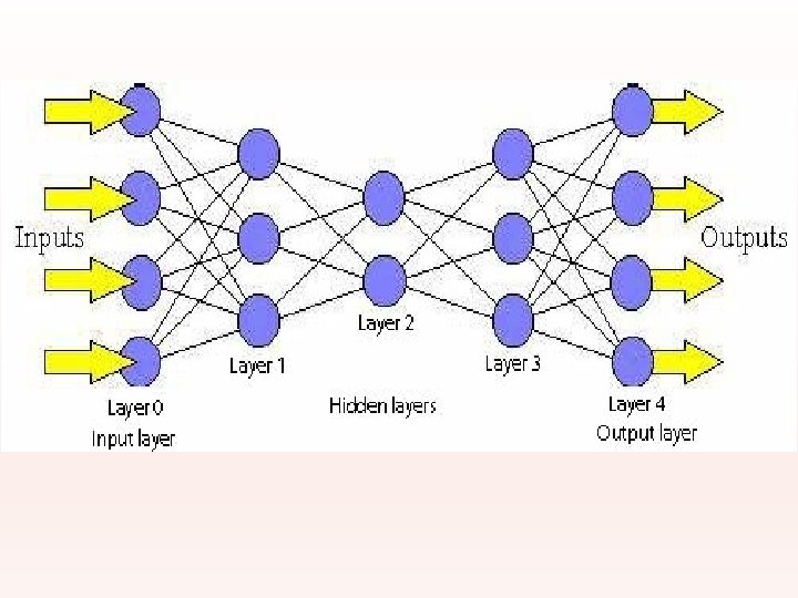
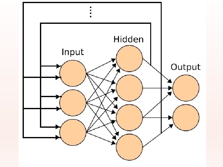
Neural Network Input Layer Hidden 1 Hidden 2 Output Layer

Network Layers The common type of ANN consists of three layers of neurons: a layer of input neurons connected to the layer of hidden neuron which is connected to a layer of output neurons.

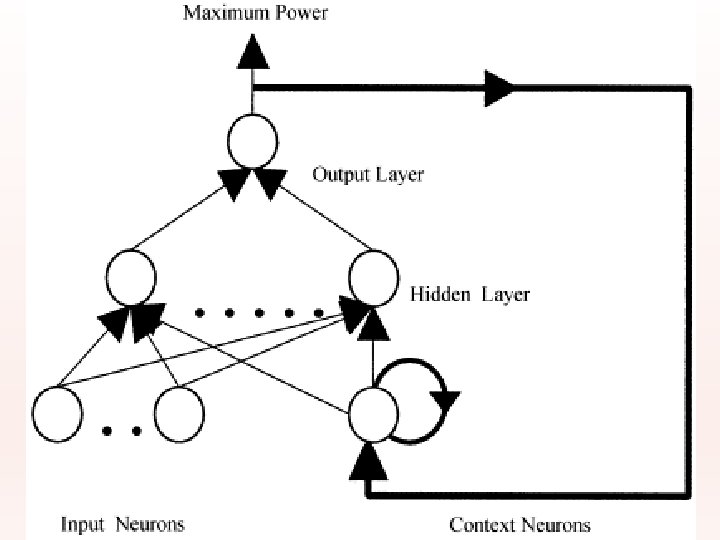
Architecture of ANN Feed-Forward networks Allow the signals to travel one way from input to output v Feed-Back Networks The signals travel as loops in the network, the output is connected to the input of the network v

How do NNs and ANNs Learn? v NNs are able to learn by adapting their connectivity patterns so that the organism improves its behavior in terms of reaching certain (evolutionary) goals. v The NN achieves learning by appropriately adapting the states of its synapses.

Neural Network Learning approach based on modeling adaptation in biological neural systems. v Perceptron: Initial algorithm for learning simple neural networks (single layer) developed in the 1950’s. v Backpropagation: More complex algorithm for learning multi-layer neural networks developed in the 1980’s. v 43

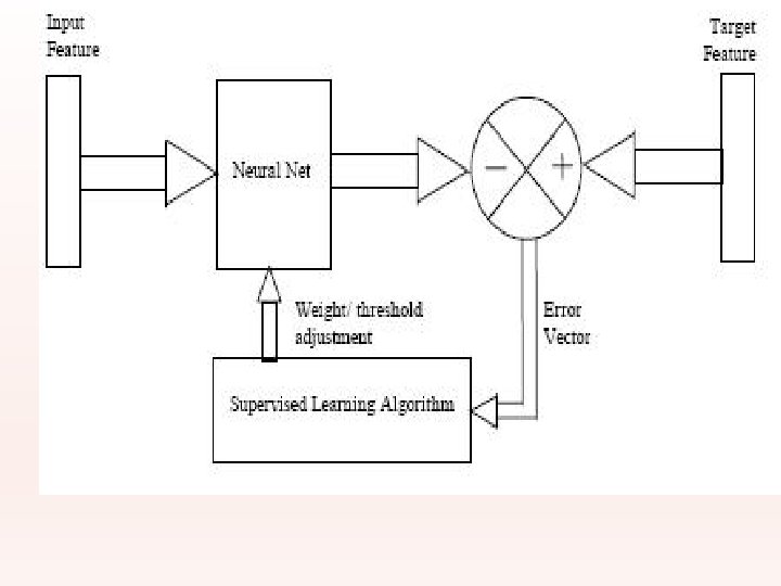
Learning Rule v The learning rule modifies the weights of the connections. v The learning process is divided into Supervised and Unsupervised learning

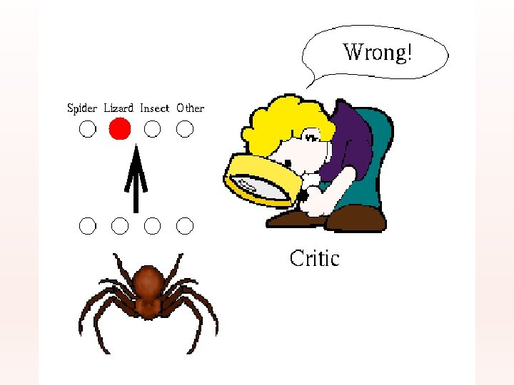
Supervised Network v Which means there exists an external teacher. The target is to minimization of the error between the desired and computed output

Unsupervised Network Uses no external teacher and is based upon only local information.

Perceptron v Perceptron is a type of artificial neural network (ANN(

Perceptron v It is a network of one neuron and hard limit transfer function X 1 W 1 Inputs X 2 Wn Xn f Output

Perceptron v The perceptron is given first a randomly weights vectors v Perceptron is given chosen data pairs (input and desired output) v Preceptron learning rule changes the weights according to the error in output

Perceptron - Operation v It takes a vector of real-valued inputs, calculates a linear combination of these inputs, then output 1 if the result is greater than some threshold and -1 otherwise

Perceptron Learning Rule W new = W old + (t-a) X Where W new is the new weight W old is the old value of weight X is the input value t is the desired value of output a is the actual value of output

Example v Let – X 1 = [0 – X 2 = [0 – X 3 = [1 – X 4 = [1 v 0] 1] and and W = [2 2] and b = -3 t =0 t=0 t=1

AND Network v This example means we construct a network for AND operation. The network draw a line to separate the classes which is called Classification

Perceptron Geometric View The equation below describes a (hyper-)plane in the input space consisting of real valued m-dimensional vectors. The plane splits the input space into two regions, each of them describing one class. decision region for C 1 x 2 w x + w >= 0 1 1 2 2 0 decision boundary C 1 C 2 x 1 w 1 x 1 + w 2 x 2 + w 0 = 0

Perceptron – Decision Surface v In 2 -dimensional space x 1 x 2 Decision Surface (Line) o=-1 o=+1 w 0 w 1 w 2

Perceptron – Representation Power v Separate the objects from the rest x 1 2 1 3 4 5 6 7 10 9 11 12 13 14 15 Elliptical blobs (objects) x 2 8 16

Problems Four one-dimensional data belonging to two classes are X = [1 -0. 5 3 -2] T = [1 -1] W = [-2. 5 1. 75] v

Boolean Functions Take in two inputs (-1 or +1) v Produce one output (-1 or +1) v In other contexts, use 0 and 1 v Example: AND function v – Produces +1 only if both inputs are +1 v Example: OR function – Produces +1 if either inputs are +1 v Related to the logical connectives from F. O. L.

The First Neural Networks X 1 1 Y X 2 1 AND Function Threshold(Y) = 2

Simple Networks -1 x y W = 1. 5 t = 0. 0 W=1

Exercises Design a neural network to recognize the problem of v X 1=[2 2] , t 1=0 v X=[1 -2], t 2=1 v X 3=[-2 2], t 3=0 v X 4=[-1 1], t 4=1 Start with initial weights w=[0 0] and bias =0 v

Perceptron: Limitations v v v The perceptron can only model linearly separable classes, like (those described by) the following Boolean functions: AND OR COMPLEMENT It cannot model the XOR You can experiment with these functions in the Matlab practical lessons.

Types of decision regions 1 Network with a single node w 0 x 1 w 1 x 2 L 1 L 2 1 1 1 Convex region L 3 w 2 x 1 L 4 x 2 1 -3. 5 1 1 One-hidden layer network that realizes the convex region

Gaussian Neurons Another type of neurons overcomes this problem by using a Gaussian activation function: fi(neti(t)) 1 0 -1 1 neti(t)

Gaussian Neurons Gaussian neurons are able to realize non-linear functions. Therefore, networks of Gaussian units are in principle unrestricted with regard to the functions that they can realize. The drawback of Gaussian neurons is that we have to make sure that their net input does not exceed 1. This adds some difficulty to the learning in Gaussian networks. 71

Sigmoidal Neurons Sigmoidal neurons accept any vectors of real numbers as input, and they output a real number between 0 and 1. Sigmoidal neurons are the most common type of artificial neuron, especially in learning networks. A network of sigmoidal units with m input neurons and n output neurons realizes a network function f: Rm (0, 1)n 72

Sigmoidal Neurons fi(neti(t)) 1 = 1 0 -1 1 neti(t) The parameter controls the slope of the sigmoid function, while the parameter controls the horizontal offset of the function in a way similar to the threshold neurons. 73

Sigmoidal Neurons This leads to a simplified form of the sigmoid function: We do not need a modifiable threshold , because we will use “dummy” inputs as we did for perceptron. The choice = 1 works well in most situations and results in a very simple derivative of S(net). 74

Sigmoidal Neurons This result will be very useful when we develop the backpropagation algorithm. 75