Machine Learning Neural Networks Human Brain Neurons InputOutput

Machine Learning Neural Networks

Human Brain

Neurons

Input-Output Transformation Input Spikes Output Spike (= a brief pulse) (Excitatory Post-Synaptic Potential)

Human Learning • • Number of neurons: Connections per neuron: Neuron switching time: Scene recognition time: ~ ~ 1010 104 to 105 0. 001 second 0. 1 second 100 inference steps doesn’t seem much

Machine Learning Abstraction

Artificial Neural Networks • Typically, machine learning ANNs are very artificial, ignoring: – Time – Space – Biological learning processes • More realistic neural models exist – Hodkins & Huxley (1952) won a Nobel prize for theirs (in 1963) • Nonetheless, very artificial ANNs have been useful in many ML applications

Perceptrons • The “first wave” in neural networks • Big in the 1960’s – Mc. Culloch & Pitts (1943), Woodrow & Hoff (1960), Rosenblatt (1962)

A single perceptron x 1 x 0 w 1 Inputs x 2 x 3 w 2 w 3 x 4 w 4 x 5 w 0 Bias (x 0 =1, always)

Logical Operators x 0 -0. 8 x 1 AND 0. 5 x 2 x 0 0. 5 0. 0 x 1 x 0 0. 5 x 2 -1. 0 -0. 3 x 1 0. 5 NOT OR

Perceptron Hypothesis Space • What’s the hypothesis space for a perceptron on n inputs?

Learning Weights • Perceptron Training Rule • Gradient Descent • (other approaches: Genetic Algorithms) x 1 x 2 x 0 ? ? ?

Perceptron Training Rule • Weights modified for each example • Update Rule: where learning rate target value perceptron output input value

What weights make XOR? x 0 ? x 1 ? x 2 ? • No combination of weights works • Perceptrons can only represent linearly separable functions

Linear Separability x 2 + + OR - + x 1

Linear Separability x 2 - + AND - - x 1

Linear Separability x 2 + XOR - + x 1

Perceptron Training Rule • Converges to the correct classification IF – Cases are linearly separable – Learning rate is slow enough – Proved by Minsky and Papert in 1969 Killed widespread interest in perceptrons till the 80’s

XOR x 0 0 0. 6 x 1 x 0 0 1 -0. 6 x 0 0 -0. 6 x 2 0. 6 1 XOR

What’s wrong with perceptrons? • You can always plug multiple perceptrons together to calculate any function. • BUT…who decides what the weights are? – Assignment of error to parental inputs becomes a problem…. – This is because of the threshold…. • Who contributed the error?

Problem: Assignment of error x 0 ? x 1 Perceptron Threshold Step function ? x 2 ? • Hard to tell from the output who contributed what • Stymies multi-layer weight learning

Solution: Differentiable Function x 0 ? x 1 Simple linear function ? x 2 ? • Varying any input a little creates a perceptible change in the output • This lets us propagate error to prior nodes

Measuring error for linear units • Output Function • Error Measure: data target value linear unit output

Gradient Descent Training rule: Gradient:

Gradient Descent Rule Update Rule:

Back to XOR x 0 x 1 XOR x 0 x 2

Gradient Descent for Multiple Layers x 0 x 1 XOR x 0 x 2 We can compute:

Gradient Descent vs. Perceptrons • Perceptron Rule & Threshold Units – Learner converges on an answer ONLY IF data is linearly separable – Can’t assign proper error to parent nodes • Gradient Descent – Minimizes error even if examples are not linearly separable – Works for multi-layer networks • But…linear units only make linear decision surfaces (can’t learn XOR even with many layers) – And the step function isn’t differentiable…

A compromise function • Perceptron • Linear • Sigmoid (Logistic)

The sigmoid (logistic) unit • Has differentiable function – Allows gradient descent • Can be used to learn non-linear functions x 1 ? x 2 ?

Logistic function Inputs Age 34 Gender 1 Stage 4 Independent variables Output. 5. 4 S . 8 Coefficients 0. 6 “Probability of being. Alive” Prediction

Neural Network Model Inputs Age Gender Stage . 6 34 2 4 Independent variables . 1. 3 . 2 . 4 S . 5. 2 S . 7 Output . 8 S . 2 Weights Hidden Layer Weights 0. 6 “Probability of being. Alive” Dependent variable Prediction

Getting an answer from a NN Inputs Age Gender 34 2 Output . 6. 5 . 1 S. 8 . 7 Stage “Probability of being. Alive” 4 Independent variables Weights Hidden Layer 0. 6 Weights Dependent variable Prediction

Getting an answer from a NN Inputs Age Output 34 . 5 . 2 Gender Stage 2 4 Independent variables S . 3 “Probability of being. Alive” . 8. 2 Weights Hidden Layer 0. 6 Weights Dependent variable Prediction

Getting an answer from a NN Inputs Age Gender Stage 34 1 4 Independent variables Output . 6. 1. 3 . 5 . 2 S. 7 “Probability of being. Alive” . 8. 2 Weights Hidden Layer 0. 6 Weights Dependent variable Prediction

Minimizing the Error surface initial error negative derivative final error local minimum winitial wtrained positive change

Differentiability is key! • Sigmoid is easy to differentiate • For gradient descent on multiple layers, a little dynamic programming can help: – Compute errors at each output node – Use these to compute errors at each hidden node – Use these to compute errors at each input node

The Backpropagation Algorithm

Getting an answer from a NN Inputs Age Gender Stage 34 1 4 Independent variables Output . 6. 1. 3 . 5 . 2 S. 7 “Probability of being. Alive” . 8. 2 Weights Hidden Layer 0. 6 Weights Dependent variable Prediction

Expressive Power of ANNs • Universal Function Approximator: – Given enough hidden units, can approximate any continuous function f • Need 2+ hidden units to learn XOR • Why not use millions of hidden units? – Efficiency (neural network training is slow) – Overfitting

Overfitting Real Distribution Overfitted Model

Combating Overfitting in Neural Nets • Many techniques • Two popular ones: – Early Stopping • Use “a lot” of hidden units • Just don’t over-train – Cross-validation • Choose the “right” number of hidden units

Early Stopping error Overfitted model errora min (Derror) a = validation set b = training set errorb Stopping criterion Epochs

Cross-validation • Cross-validation: general-purpose technique for model selection – E. g. , “how many hidden units should I use? ” • More extensive version of validation-set approach.

Cross-validation • Break training set into k sets • For each model M – For i=1…k • Train M on all but set i • Test on set i • Output M with highest average test score, trained on full training set

Summary of Neural Networks Non-linear regression technique that is trained with gradient descent. Question: How important is the biological metaphor?

Summary of Neural Networks When are Neural Networks useful? – Instances represented by attribute-value pairs • Particularly when attributes are real valued – The target function is • Discrete-valued • Real-valued • Vector-valued – Training examples may contain errors – Fast evaluation times are necessary When not? – Fast training times are necessary – Understandability of the function is required

Advanced Topics in Neural Nets • • • Batch Move vs. incremental Hidden Layer Representations Hopfield Nets Neural Networks on Silicon Neural Network language models

Incremental vs. Batch Mode

Incremental vs. Batch Mode • In Batch Mode we minimize: • Same as computing: • Then setting

Advanced Topics in Neural Nets • • • Batch Move vs. incremental Hidden Layer Representations Hopfield Nets Neural Networks on Silicon Neural Network language models

Hidden Layer Representations • Input->Hidden Layer mapping: – representation of input vectors tailored to the task • Can also be exploited for dimensionality reduction – Form of unsupervised learning in which we output a “more compact” representation of input vectors – <x 1, …, xn> -> <x’ 1, …, x’m> where m < n – Useful for visualization, problem simplification, data compression, etc.

Dimensionality Reduction Model: Function to learn:

Dimensionality Reduction: Example

Advanced Topics in Neural Nets • • • Batch Move vs. incremental Hidden Layer Representations Hopfield Nets Neural Networks on Silicon Neural Network language models

Neural Networks on Silicon • Currently: Simulation of continuous device physics (neural networks) Digital computational model Why not (thresholding) skip this? Continuous device physics (voltage)

Example: Silicon Retina Simulates function of biological retina Single-transistor synapses adapt to luminance, temporal contrast Modeling retina directly on chip => requires 100 x less power!

Example: Silicon Retina • Synapses modeled with single transistors

Luminance Adaptation

Comparison with Mammal Data • Real: • Artificial:

• Graphics and results taken from:

General NN learning in silicon? • Seems less in-vogue than in late-90 s • Interest has turned somewhat to implementing Bayesian techniques in analog silicon

Advanced Topics in Neural Nets • • • Batch Move vs. incremental Hidden Layer Representations Hopfield Nets Neural Networks on Silicon Neural Network language models

Neural Network Language Models • Statistical Language Modeling: – Predict probability of next word in sequence I was headed to Madrid , ____ P(___ = “Spain”) = 0. 5, P(___ = “but”) = 0. 2, etc. • Used in speech recognition, machine translation, (recently) information extraction

Formally • Estimate:

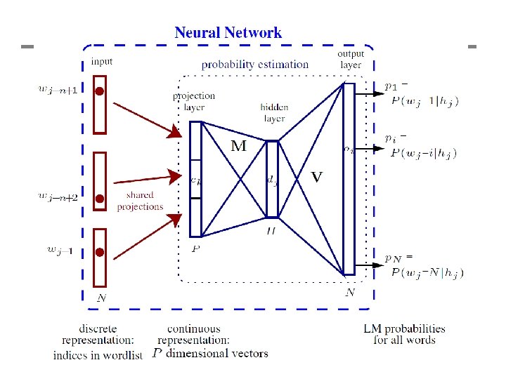
Optimizations • Key idea – learn simultaneously: – vector representations for each word (50 dim) – a predictor of the next word • Short-lists – Much complexity in hidden->output layer • Number of possible next words is large – Only predict a subset of words • Use a standard probabilistic model for the rest

Design Decisions (1) • Number of hidden units • Almost no difference…

Design Decisions (2) • Word representation (# of dimensions) • They chose 120

Comparison vs. state of the art