Machine Learning Mixture Model HMM and Expectation Maximization

Machine Learning Mixture Model, HMM, and Expectation Maximization Eric Xing Lecture 9, August 14, 2010 Reading: Eric Xing © Eric Xing @ CMU, 2006 -2010

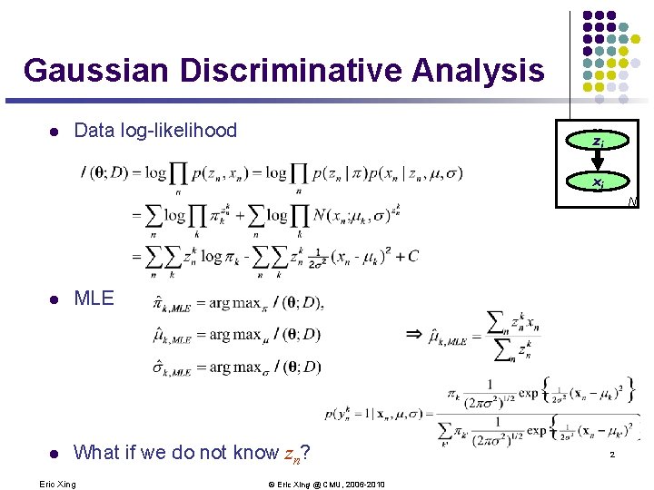
Gaussian Discriminative Analysis l Data log-likelihood zi xi N l MLE l What if we do not know zn? Eric Xing © Eric Xing @ CMU, 2006 -2010 2

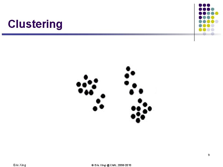
Clustering 3 Eric Xing © Eric Xing @ CMU, 2006 -2010

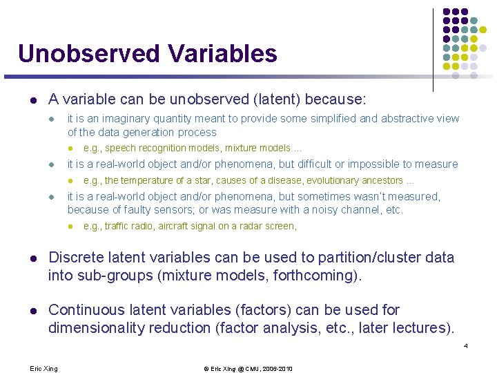
Unobserved Variables l A variable can be unobserved (latent) because: l it is an imaginary quantity meant to provide some simplified and abstractive view of the data generation process l l it is a real-world object and/or phenomena, but difficult or impossible to measure l l e. g. , speech recognition models, mixture models … e. g. , the temperature of a star, causes of a disease, evolutionary ancestors … it is a real-world object and/or phenomena, but sometimes wasn’t measured, because of faulty sensors; or was measure with a noisy channel, etc. l e. g. , traffic radio, aircraft signal on a radar screen, l Discrete latent variables can be used to partition/cluster data into sub-groups (mixture models, forthcoming). l Continuous latent variables (factors) can be used for dimensionality reduction (factor analysis, etc. , later lectures). 4 Eric Xing © Eric Xing @ CMU, 2006 -2010

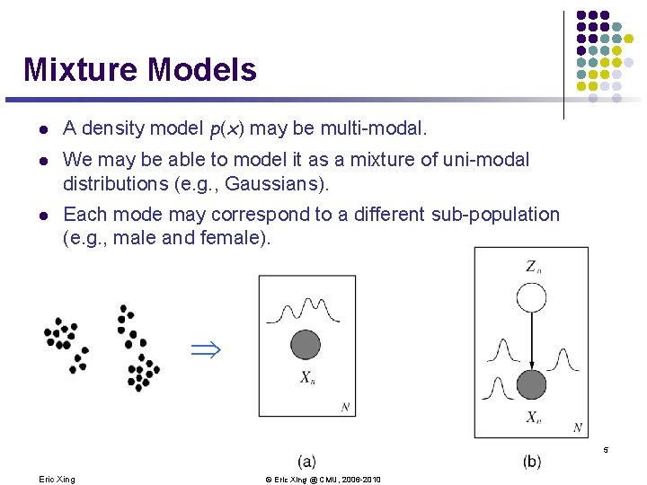
Mixture Models l A density model p(x) may be multi-modal. l We may be able to model it as a mixture of uni-modal distributions (e. g. , Gaussians). l Each mode may correspond to a different sub-population (e. g. , male and female). Þ 5 Eric Xing © Eric Xing @ CMU, 2006 -2010

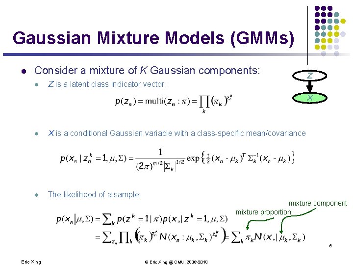
Gaussian Mixture Models (GMMs) l Consider a mixture of K Gaussian components: l Z is a latent class indicator vector: Z X l X is a conditional Gaussian variable with a class-specific mean/covariance l The likelihood of a sample: mixture component mixture proportion 6 Eric Xing © Eric Xing @ CMU, 2006 -2010

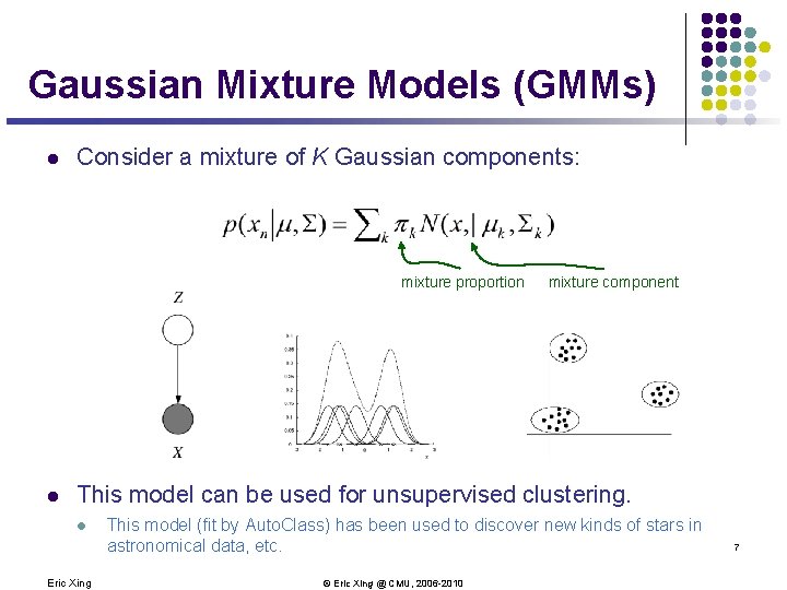
Gaussian Mixture Models (GMMs) l Consider a mixture of K Gaussian components: mixture proportion l mixture component This model can be used for unsupervised clustering. l Eric Xing This model (fit by Auto. Class) has been used to discover new kinds of stars in astronomical data, etc. © Eric Xing @ CMU, 2006 -2010 7

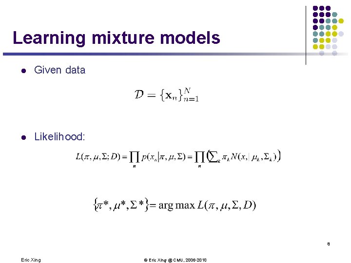
Learning mixture models l Given data l Likelihood: 8 Eric Xing © Eric Xing @ CMU, 2006 -2010

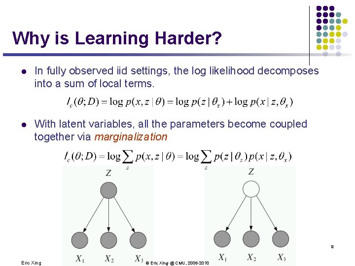
Why is Learning Harder? l In fully observed iid settings, the log likelihood decomposes into a sum of local terms. l With latent variables, all the parameters become coupled together via marginalization 9 Eric Xing © Eric Xing @ CMU, 2006 -2010

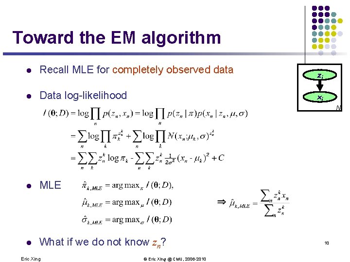
Toward the EM algorithm l Recall MLE for completely observed data l Data log-likelihood zi xi N l MLE l What if we do not know zn? Eric Xing © Eric Xing @ CMU, 2006 -2010 10

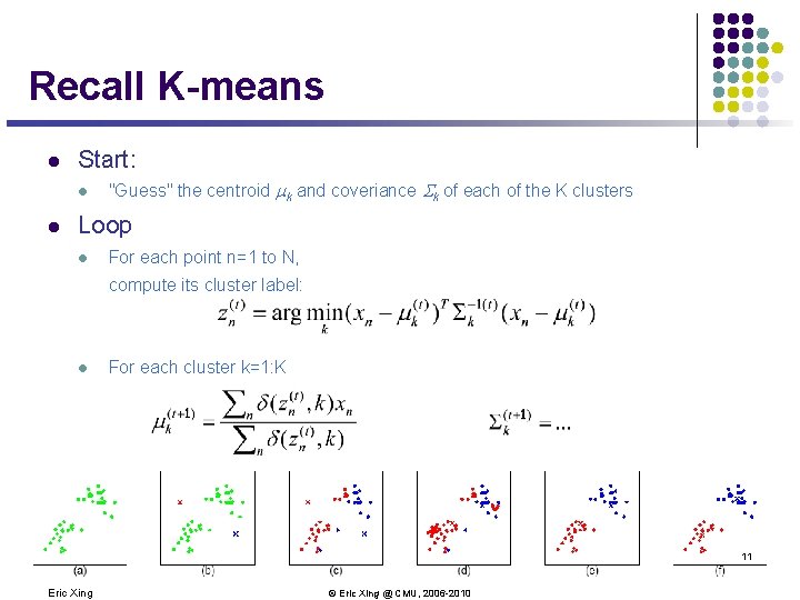
Recall K-means l Start: l l "Guess" the centroid mk and coveriance Sk of each of the K clusters Loop l For each point n=1 to N, compute its cluster label: l For each cluster k=1: K 11 Eric Xing © Eric Xing @ CMU, 2006 -2010

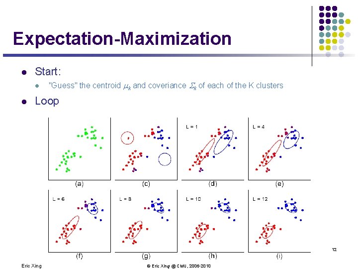
Expectation-Maximization l Start: l l "Guess" the centroid mk and coveriance Sk of each of the K clusters Loop 12 Eric Xing © Eric Xing @ CMU, 2006 -2010

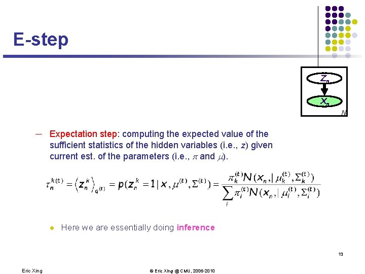
E-step Zn Xn N ─ Expectation step: computing the expected value of the sufficient statistics of the hidden variables (i. e. , z) given current est. of the parameters (i. e. , p and m). l Here we are essentially doing inference 13 Eric Xing © Eric Xing @ CMU, 2006 -2010

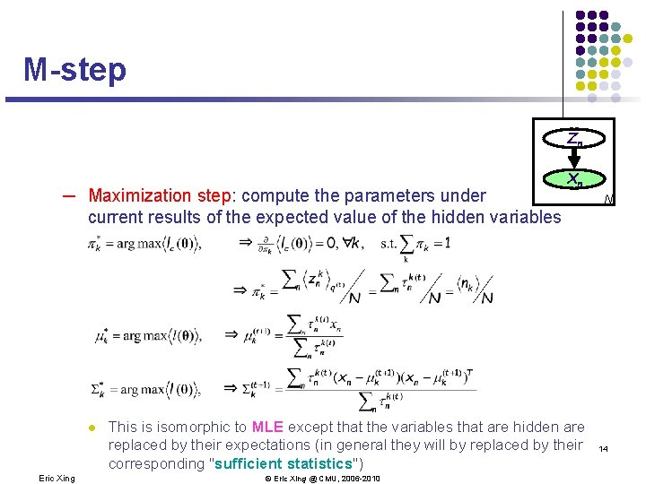
M-step Zn ─ Maximization step: compute the parameters under current results of the expected value of the hidden variables l Eric Xing Xn This is isomorphic to MLE except that the variables that are hidden are replaced by their expectations (in general they will by replaced by their corresponding "sufficient statistics") © Eric Xing @ CMU, 2006 -2010 N 14

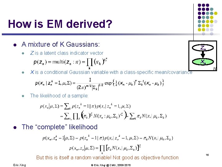
How is EM derived? l A mixture of K Gaussians: l Z is a latent class indicator vector Zn Xn l l X is a conditional Gaussian variable with a class-specific mean/covariance l The likelihood of a sample: N The “complete” likelihood But this is itself a random variable! Not good as objective function Eric Xing © Eric Xing @ CMU, 2006 -2010 15

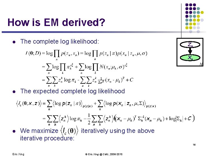
How is EM derived? l The complete log likelihood: Zn Xn N l The expected complete log likelihood l We maximize iterative procedure: iteratively using the above 16 Eric Xing © Eric Xing @ CMU, 2006 -2010

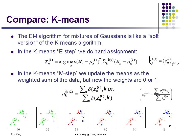
Compare: K-means l The EM algorithm for mixtures of Gaussians is like a "soft version" of the K-means algorithm. l In the K-means “E-step” we do hard assignment: l In the K-means “M-step” we update the means as the weighted sum of the data, but now the weights are 0 or 1: 17 Eric Xing © Eric Xing @ CMU, 2006 -2010

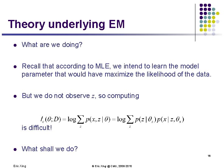
Theory underlying EM l What are we doing? l Recall that according to MLE, we intend to learn the model parameter that would have maximize the likelihood of the data. l But we do not observe z, so computing is difficult! l What shall we do? 18 Eric Xing © Eric Xing @ CMU, 2006 -2010

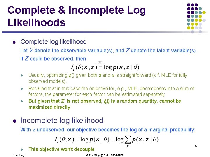
Complete & Incomplete Log Likelihoods l Complete log likelihood Let X denote the observable variable(s), and Z denote the latent variable(s). If Z could be observed, then l l Usually, optimizing lc() given both z and x is straightforward (c. f. MLE for fully observed models). Recalled that in this case the objective for, e. g. , MLE, decomposes into a sum of factors, the parameter for each factor can be estimated separately. But given that Z is not observed, lc() is a random quantity, cannot be maximized directly. Incomplete log likelihood With z unobserved, our objective becomes the log of a marginal probability: l Eric Xing This objective won't decouple © Eric Xing @ CMU, 2006 -2010 19

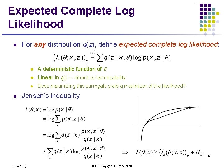
Expected Complete Log Likelihood l For any distribution q(z), define expected complete log likelihood: l A deterministic function of Linear in lc() --- inherit its factorizabiility l Does maximizing this surrogate yield a maximizer of the likelihood? l l Jensen’s inequality 20 Eric Xing © Eric Xing @ CMU, 2006 -2010

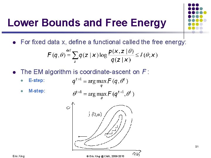
Lower Bounds and Free Energy l For fixed data x, define a functional called the free energy: l The EM algorithm is coordinate-ascent on F : l E-step: l M-step: 21 Eric Xing © Eric Xing @ CMU, 2006 -2010

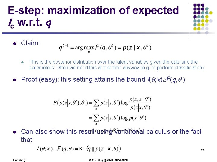
E-step: maximization of expected lc w. r. t. q l Claim: l l l This is the posterior distribution over the latent variables given the data and the parameters. Often we need this at test time anyway (e. g. to perform classification). Proof (easy): this setting attains the bound l( ; x)³F(q, ) Can also show this result using variational calculus or the fact that 22 Eric Xing © Eric Xing @ CMU, 2006 -2010

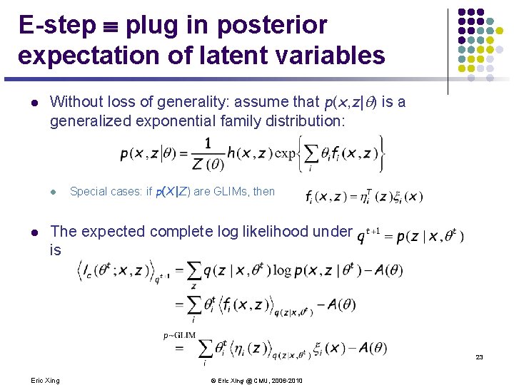
E-step º plug in posterior expectation of latent variables l Without loss of generality: assume that p(x, z| ) is a generalized exponential family distribution: l l Special cases: if p(X|Z) are GLIMs, then The expected complete log likelihood under is 23 Eric Xing © Eric Xing @ CMU, 2006 -2010

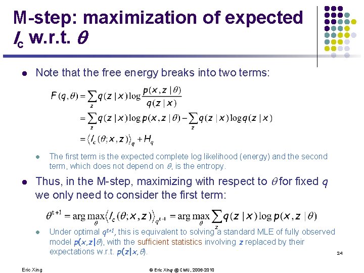
M-step: maximization of expected lc w. r. t. l Note that the free energy breaks into two terms: l l The first term is the expected complete log likelihood (energy) and the second term, which does not depend on , is the entropy. Thus, in the M-step, maximizing with respect to for fixed q we only need to consider the first term: l Eric Xing Under optimal qt+1, this is equivalent to solving a standard MLE of fully observed model p(x, z| ), with the sufficient statistics involving z replaced by their expectations w. r. t. p(z|x, ). 24 © Eric Xing @ CMU, 2006 -2010

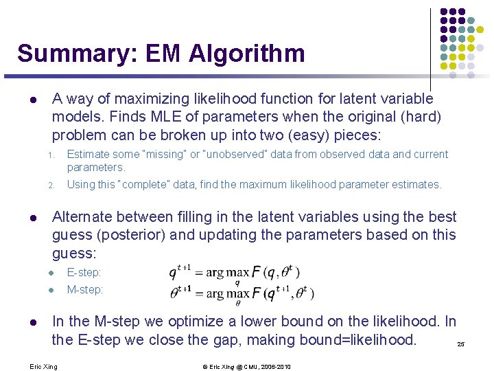
Summary: EM Algorithm l l l A way of maximizing likelihood function for latent variable models. Finds MLE of parameters when the original (hard) problem can be broken up into two (easy) pieces: 1. Estimate some “missing” or “unobserved” data from observed data and current parameters. 2. Using this “complete” data, find the maximum likelihood parameter estimates. Alternate between filling in the latent variables using the best guess (posterior) and updating the parameters based on this guess: l E-step: l M-step: In the M-step we optimize a lower bound on the likelihood. In the E-step we close the gap, making bound=likelihood. 25 Eric Xing © Eric Xing @ CMU, 2006 -2010

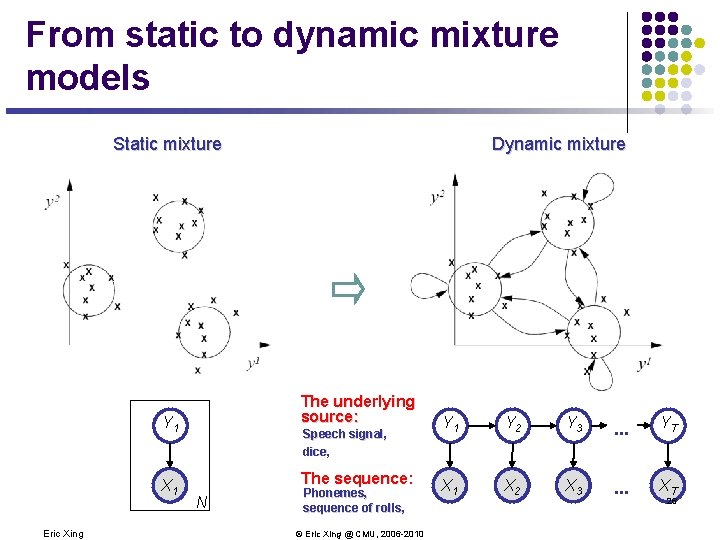
From static to dynamic mixture models Static mixture The underlying source: Y 1 A 1 X Eric Xing Dynamic mixture Speech signal, dice, The sequence: N Phonemes, sequence of rolls, © Eric Xing @ CMU, 2006 -2010 Y 1 Y 2 Y 3 . . . YT A 1 X A 2 X A 3 X . . . XAT 26

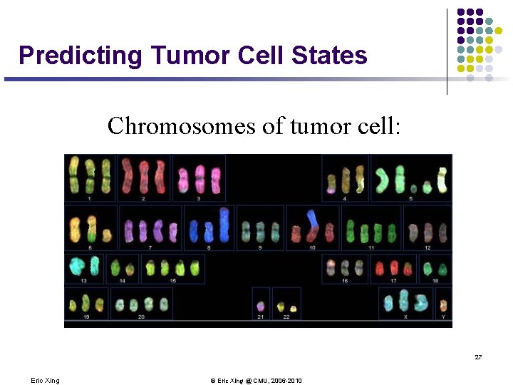
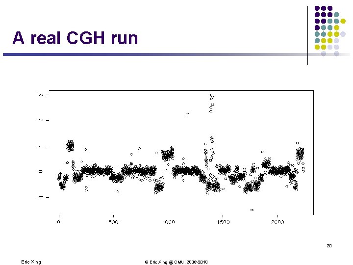
Predicting Tumor Cell States Chromosomes of tumor cell: 27 Eric Xing © Eric Xing @ CMU, 2006 -2010

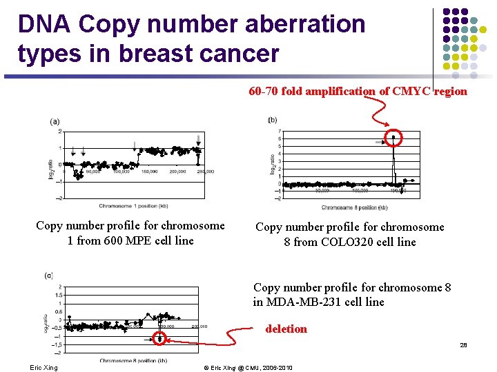
DNA Copy number aberration types in breast cancer 60 -70 fold amplification of CMYC region Copy number profile for chromosome 1 from 600 MPE cell line Copy number profile for chromosome 8 from COLO 320 cell line Copy number profile for chromosome 8 in MDA-MB-231 cell line deletion 28 Eric Xing © Eric Xing @ CMU, 2006 -2010

A real CGH run 29 Eric Xing © Eric Xing @ CMU, 2006 -2010

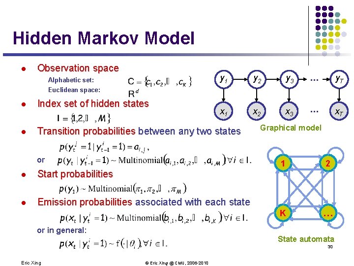
Hidden Markov Model l Observation space Alphabetic set: y 1 y 2 y 3 . . . y. T x. A 1 x. A 2 x. A 3 . . . x. AT Euclidean space: l Index set of hidden states l Transition probabilities between any two states or l Start probabilities l Emission probabilities associated with each state or in general: Graphical model 1 2 K … State automata 30 Eric Xing © Eric Xing @ CMU, 2006 -2010

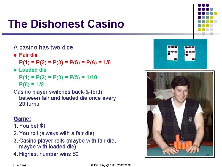
The Dishonest Casino A casino has two dice: Fair die P(1) = P(2) = P(3) = P(5) = P(6) = 1/6 l Loaded die P(1) = P(2) = P(3) = P(5) = 1/10 P(6) = 1/2 Casino player switches back-&-forth between fair and loaded die once every 20 turns l Game: 1. You bet $1 2. You roll (always with a fair die) 3. Casino player rolls (maybe with fair die, maybe with loaded die) 4. Highest number wins $2 Eric Xing © Eric Xing @ CMU, 2006 -2010 31

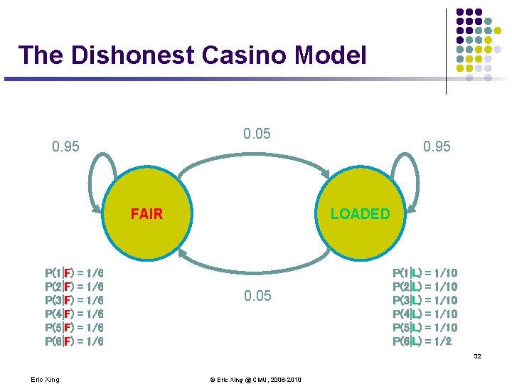
The Dishonest Casino Model 0. 05 0. 95 FAIR P(1|F) P(2|F) P(3|F) P(4|F) P(5|F) P(6|F) = = = 1/6 1/6 1/6 0. 95 LOADED 0. 05 P(1|L) P(2|L) P(3|L) P(4|L) P(5|L) P(6|L) = = = 1/10 1/10 1/2 32 Eric Xing © Eric Xing @ CMU, 2006 -2010

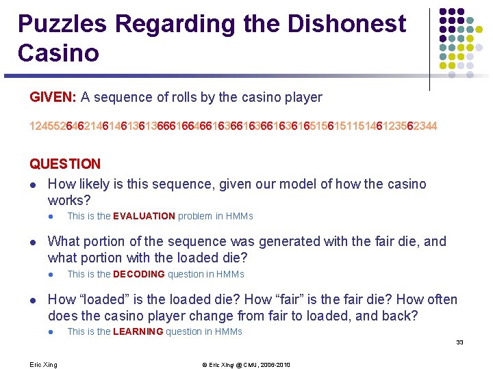
Puzzles Regarding the Dishonest Casino GIVEN: A sequence of rolls by the casino player 12455264621461461361366616646616366163616515615115146123562344 QUESTION l How likely is this sequence, given our model of how the casino works? l l What portion of the sequence was generated with the fair die, and what portion with the loaded die? l l This is the EVALUATION problem in HMMs This is the DECODING question in HMMs How “loaded” is the loaded die? How “fair” is the fair die? How often does the casino player change from fair to loaded, and back? l This is the LEARNING question in HMMs 33 Eric Xing © Eric Xing @ CMU, 2006 -2010

Joint Probability 12455264621461461361366616646616366163616515615115146123562344 34 Eric Xing © Eric Xing @ CMU, 2006 -2010

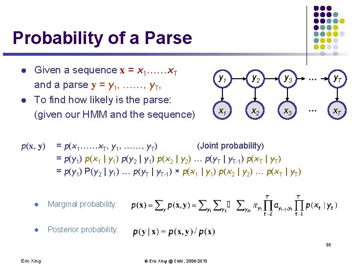
Probability of a Parse l l Given a sequence x = x 1……x. T and a parse y = y 1, ……, y. T, To find how likely is the parse: (given our HMM and the sequence) p(x, y) y 1 y 2 y 3 . . . y. T x. A 1 x. A 2 x. A 3 . . . x. AT = p(x 1……x. T, y 1, ……, y. T) (Joint probability) = p(y 1) p(x 1 | y 1) p(y 2 | y 1) p(x 2 | y 2) … p(y. T | y. T-1) p(x. T | y. T) = p(y 1) P(y 2 | y 1) … p(y. T | y. T-1) × p(x 1 | y 1) p(x 2 | y 2) … p(x. T | y. T) l Marginal probability: l Posterior probability: 35 Eric Xing © Eric Xing @ CMU, 2006 -2010

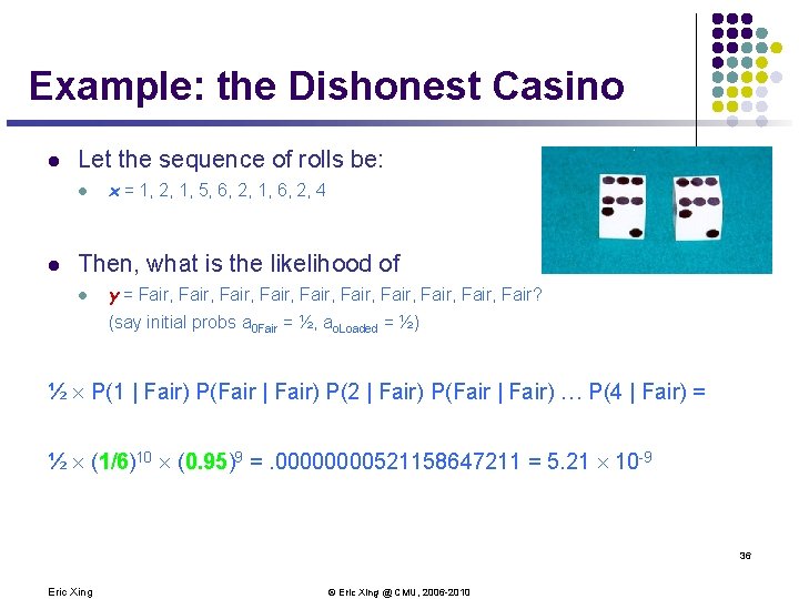
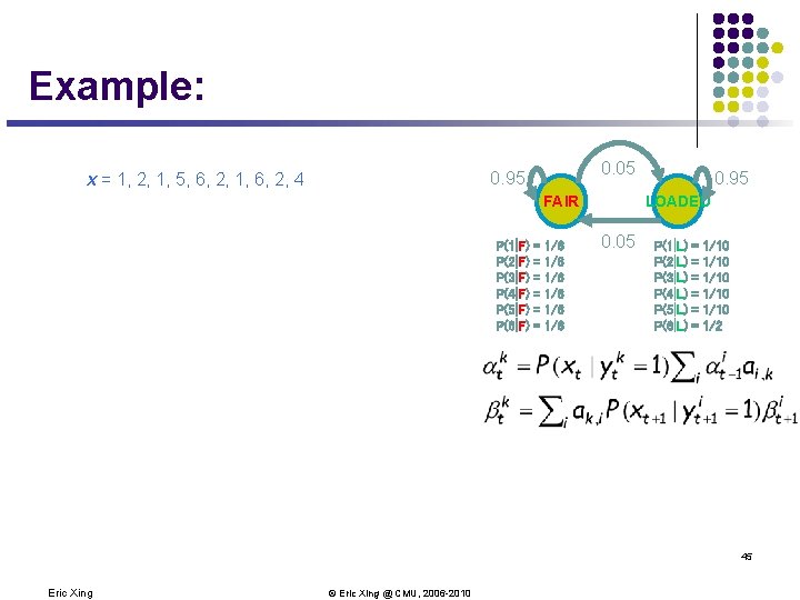
Example: the Dishonest Casino l Let the sequence of rolls be: l l x = 1, 2, 1, 5, 6, 2, 1, 6, 2, 4 Then, what is the likelihood of l y = Fair, Fair, Fair, Fair? (say initial probs a 0 Fair = ½, ao. Loaded = ½) ½ P(1 | Fair) P(Fair | Fair) P(2 | Fair) P(Fair | Fair) … P(4 | Fair) = ½ (1/6)10 (0. 95)9 =. 0000521158647211 = 5. 21 10 -9 36 Eric Xing © Eric Xing @ CMU, 2006 -2010

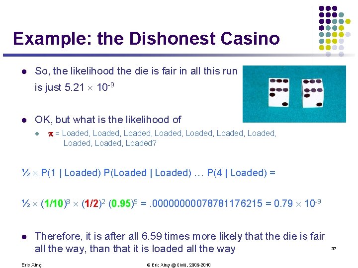
Example: the Dishonest Casino l So, the likelihood the die is fair in all this run is just 5. 21 10 -9 l OK, but what is the likelihood of l = Loaded, Loaded, Loaded, Loaded? ½ P(1 | Loaded) P(Loaded | Loaded) … P(4 | Loaded) = ½ (1/10)8 (1/2)2 (0. 95)9 =. 0000078781176215 = 0. 79 10 -9 l Therefore, it is after all 6. 59 times more likely that the die is fair all the way, than that it is loaded all the way Eric Xing © Eric Xing @ CMU, 2006 -2010 37

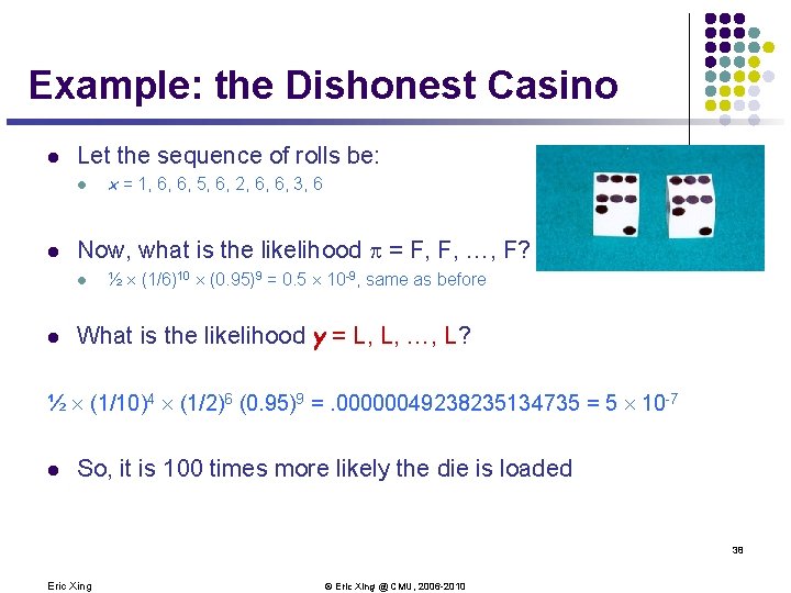
Example: the Dishonest Casino l Let the sequence of rolls be: l l Now, what is the likelihood = F, F, …, F? l l x = 1, 6, 6, 5, 6, 2, 6, 6, 3, 6 ½ (1/6)10 (0. 95)9 = 0. 5 10 -9, same as before What is the likelihood y = L, L, …, L? ½ (1/10)4 (1/2)6 (0. 95)9 =. 00000049238235134735 = 5 10 -7 l So, it is 100 times more likely the die is loaded 38 Eric Xing © Eric Xing @ CMU, 2006 -2010

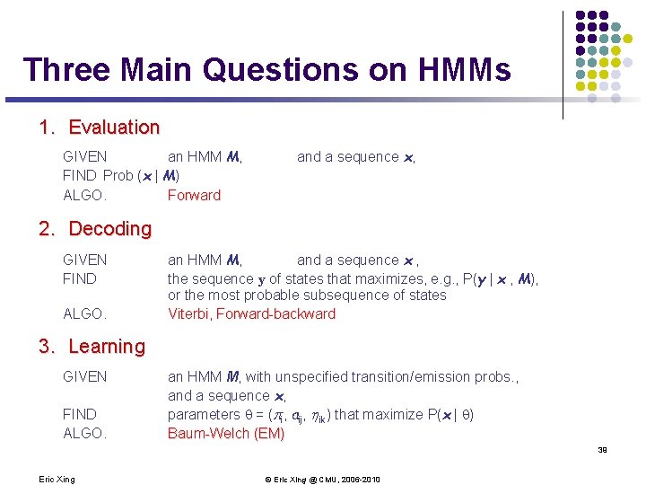
Three Main Questions on HMMs 1. Evaluation GIVEN an HMM M, FIND Prob (x | M) ALGO. Forward and a sequence x, 2. Decoding GIVEN FIND ALGO. an HMM M, and a sequence x , the sequence y of states that maximizes, e. g. , P(y | x , M), or the most probable subsequence of states Viterbi, Forward-backward 3. Learning GIVEN FIND ALGO. an HMM M, with unspecified transition/emission probs. , and a sequence x, parameters = (pi, aij, hik) that maximize P(x | ) Baum-Welch (EM) 39 Eric Xing © Eric Xing @ CMU, 2006 -2010

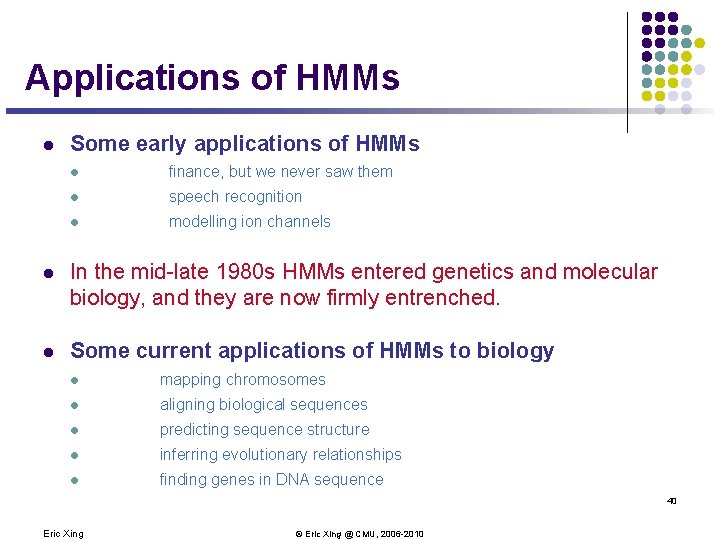
Applications of HMMs l Some early applications of HMMs l finance, but we never saw them l speech recognition l modelling ion channels l In the mid-late 1980 s HMMs entered genetics and molecular biology, and they are now firmly entrenched. l Some current applications of HMMs to biology l mapping chromosomes l aligning biological sequences l predicting sequence structure l inferring evolutionary relationships l finding genes in DNA sequence 40 Eric Xing © Eric Xing @ CMU, 2006 -2010

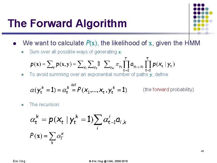
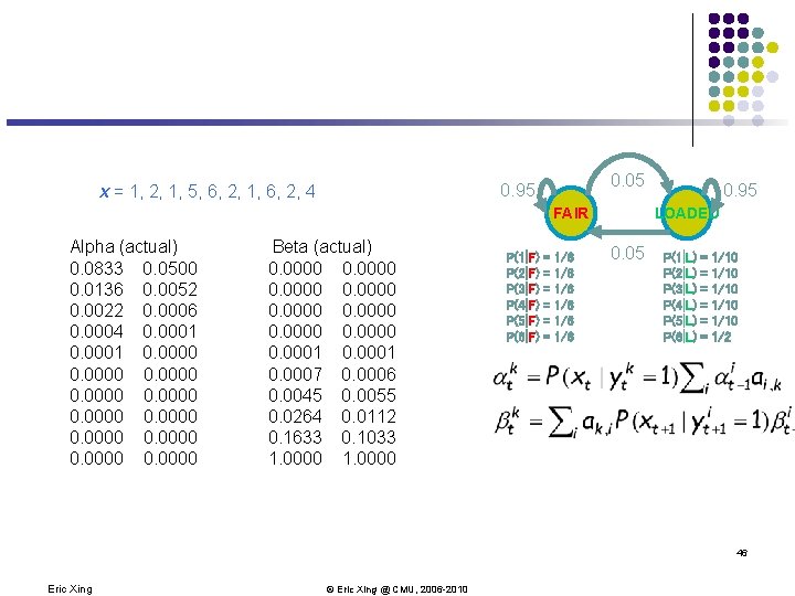
The Forward Algorithm l We want to calculate P(x), the likelihood of x, given the HMM l Sum over all possible ways of generating x: l To avoid summing over an exponential number of paths y, define (the forward probability) l The recursion: 41 Eric Xing © Eric Xing @ CMU, 2006 -2010

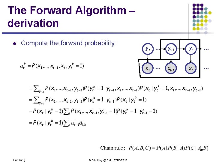
The Forward Algorithm – derivation l Compute the forward probability: y 1 . . . yt-1 yt . . . x. A 1 . . . x. A t-1 xt A . . . 42 Eric Xing © Eric Xing @ CMU, 2006 -2010

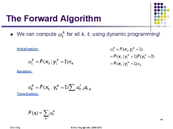
The Forward Algorithm l We can compute for all k, t, using dynamic programming! Initialization: Iteration: Termination: 43 Eric Xing © Eric Xing @ CMU, 2006 -2010

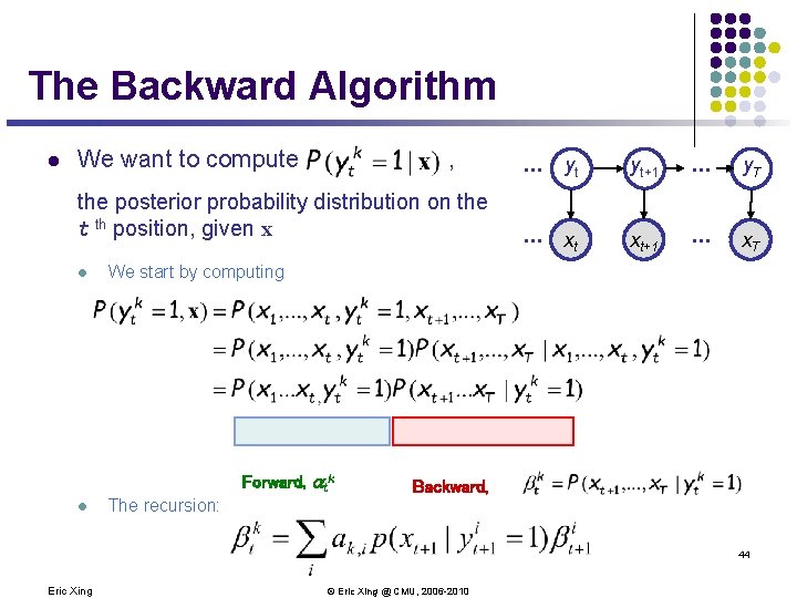
The Backward Algorithm l We want to compute , the posterior probability distribution on the t th position, given x l yt yt+1 . . . y. T . . . A xt x. A t+1 . . . x. AT We start by computing Forward, atk l . . . Backward, The recursion: 44 Eric Xing © Eric Xing @ CMU, 2006 -2010

Example: 0. 05 0. 95 x = 1, 2, 1, 5, 6, 2, 1, 6, 2, 4 FAIR P(1|F) P(2|F) P(3|F) P(4|F) P(5|F) P(6|F) = = = 1/6 1/6 1/6 0. 95 LOADED 0. 05 P(1|L) P(2|L) P(3|L) P(4|L) P(5|L) P(6|L) = = = 1/10 1/10 1/2 45 Eric Xing © Eric Xing @ CMU, 2006 -2010

0. 05 0. 95 x = 1, 2, 1, 5, 6, 2, 1, 6, 2, 4 FAIR Alpha (actual) 0. 0833 0. 0500 0. 0136 0. 0052 0. 0022 0. 0006 0. 0004 0. 0001 0. 0000 0. 0000 Beta (actual) 0. 0000 0. 0001 0. 0007 0. 0006 0. 0045 0. 0055 0. 0264 0. 0112 0. 1633 0. 1033 1. 0000 P(1|F) P(2|F) P(3|F) P(4|F) P(5|F) P(6|F) = = = 1/6 1/6 1/6 0. 95 LOADED 0. 05 P(1|L) P(2|L) P(3|L) P(4|L) P(5|L) P(6|L) = = = 1/10 1/10 1/2 46 Eric Xing © Eric Xing @ CMU, 2006 -2010

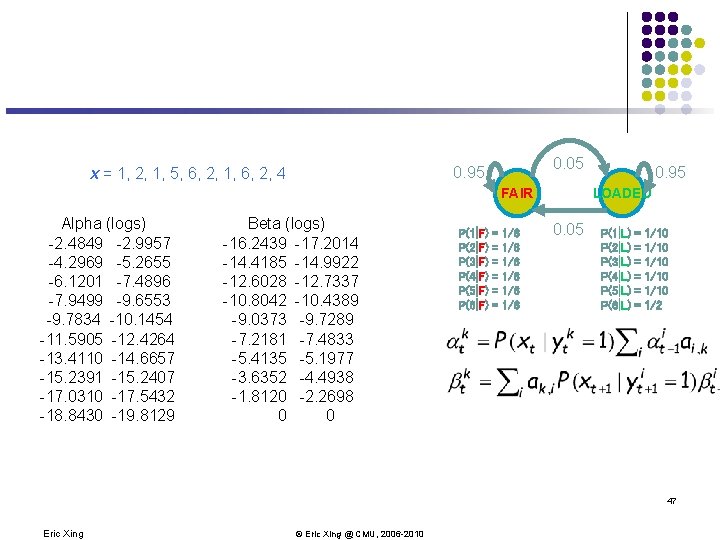
0. 05 0. 95 x = 1, 2, 1, 5, 6, 2, 1, 6, 2, 4 FAIR Alpha (logs) -2. 4849 -2. 9957 -4. 2969 -5. 2655 -6. 1201 -7. 4896 -7. 9499 -9. 6553 -9. 7834 -10. 1454 -11. 5905 -12. 4264 -13. 4110 -14. 6657 -15. 2391 -15. 2407 -17. 0310 -17. 5432 -18. 8430 -19. 8129 Beta (logs) -16. 2439 -17. 2014 -14. 4185 -14. 9922 -12. 6028 -12. 7337 -10. 8042 -10. 4389 -9. 0373 -9. 7289 -7. 2181 -7. 4833 -5. 4135 -5. 1977 -3. 6352 -4. 4938 -1. 8120 -2. 2698 0 0 P(1|F) P(2|F) P(3|F) P(4|F) P(5|F) P(6|F) = = = 1/6 1/6 1/6 0. 95 LOADED 0. 05 P(1|L) P(2|L) P(3|L) P(4|L) P(5|L) P(6|L) = = = 1/10 1/10 1/2 47 Eric Xing © Eric Xing @ CMU, 2006 -2010

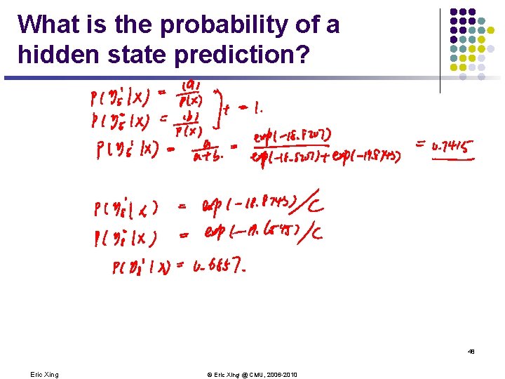
What is the probability of a hidden state prediction? 48 Eric Xing © Eric Xing @ CMU, 2006 -2010

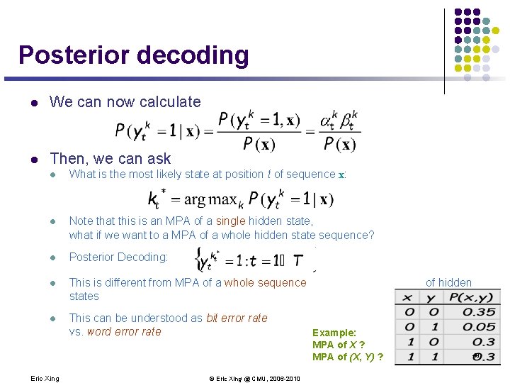
Posterior decoding l We can now calculate l Then, we can ask l What is the most likely state at position t of sequence x: l Note that this is an MPA of a single hidden state, what if we want to a MPA of a whole hidden state sequence? l Posterior Decoding: l This is different from MPA of a whole sequence states l This can be understood as bit error rate vs. word error rate Eric Xing © Eric Xing @ CMU, 2006 -2010 of hidden Example: MPA of X ? MPA of (X, Y) ? 49

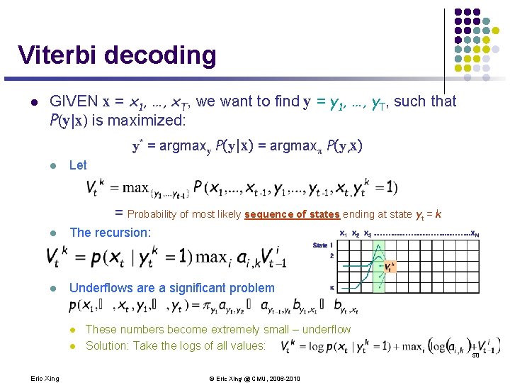
Viterbi decoding l GIVEN x = x 1, …, x. T, we want to find y = y 1, …, y. T, such that P(y|x) is maximized: y* = argmaxy P(y|x) = argmax P(y, x) l Let = Probability of most likely sequence of states ending at state yt = k l The recursion: l Underflows are a significant problem l l These numbers become extremely small – underflow Solution: Take the logs of all values: 50 Eric Xing © Eric Xing @ CMU, 2006 -2010

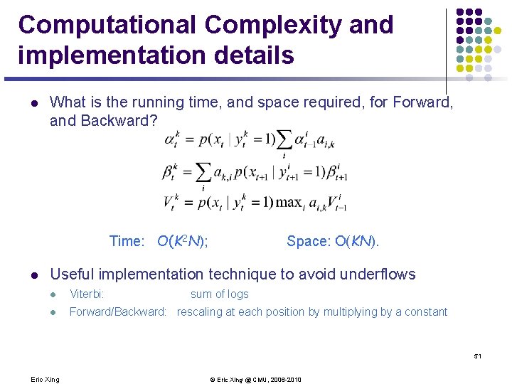
Computational Complexity and implementation details l What is the running time, and space required, for Forward, and Backward? Time: O(K 2 N); l Space: O(KN). Useful implementation technique to avoid underflows l Viterbi: sum of logs l Forward/Backward: rescaling at each position by multiplying by a constant 51 Eric Xing © Eric Xing @ CMU, 2006 -2010

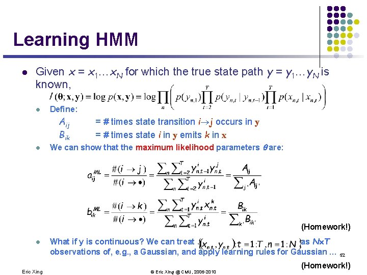
Learning HMM l Given x = x 1…x. N for which the true state path y = y 1…y. N is known, l Define: Aij Bik l = # times state transition i j occurs in y = # times state i in y emits k in x We can show that the maximum likelihood parameters are: (Homework!) l Eric Xing What if y is continuous? We can treat as N´T observations of, e. g. , a Gaussian, and apply learning rules for Gaussian … 52 © Eric Xing @ CMU, 2006 -2010 (Homework!)

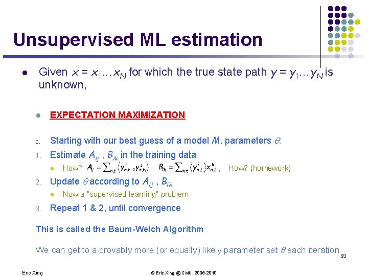
Unsupervised ML estimation l Given x = x 1…x. N for which the true state path y = y 1…y. N is unknown, l EXPECTATION MAXIMIZATION 0. Starting with our best guess of a model M, parameters : 1. Estimate Aij , Bik in the training data l 2. , , How? (homework) Update according to Aij , Bik l 3. How? Now a "supervised learning" problem Repeat 1 & 2, until convergence This is called the Baum-Welch Algorithm We can get to a provably more (or equally) likely parameter set each iteration Eric Xing © Eric Xing @ CMU, 2006 -2010 53

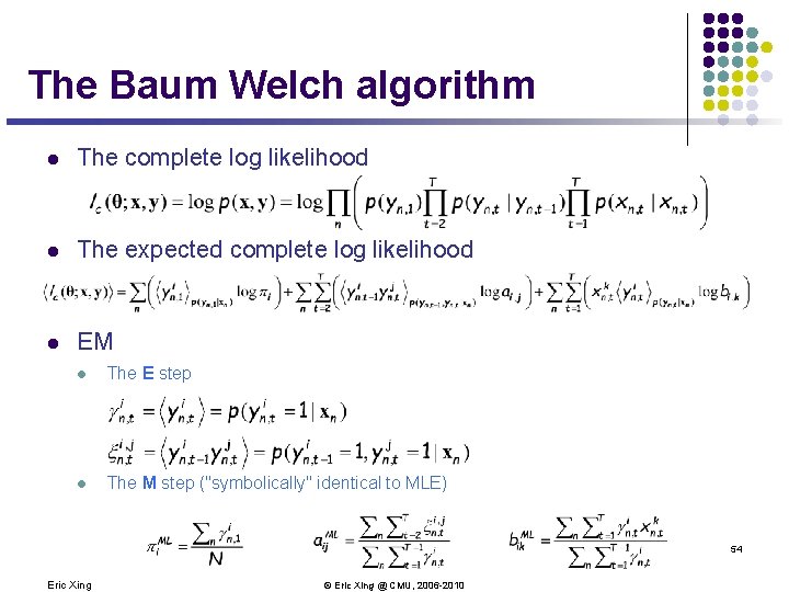
The Baum Welch algorithm l The complete log likelihood l The expected complete log likelihood l EM l The E step l The M step ("symbolically" identical to MLE) 54 Eric Xing © Eric Xing @ CMU, 2006 -2010

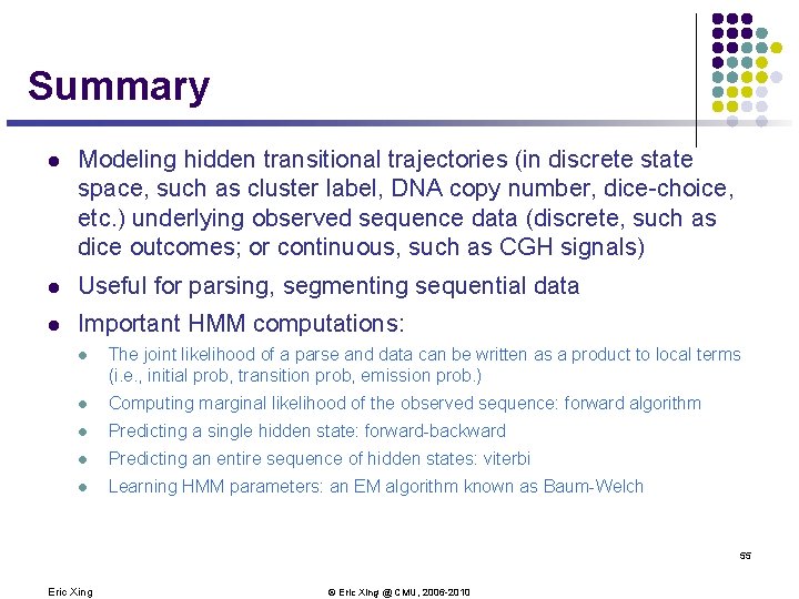
Summary l Modeling hidden transitional trajectories (in discrete state space, such as cluster label, DNA copy number, dice-choice, etc. ) underlying observed sequence data (discrete, such as dice outcomes; or continuous, such as CGH signals) l Useful for parsing, segmenting sequential data l Important HMM computations: l The joint likelihood of a parse and data can be written as a product to local terms (i. e. , initial prob, transition prob, emission prob. ) l Computing marginal likelihood of the observed sequence: forward algorithm l Predicting a single hidden state: forward-backward l Predicting an entire sequence of hidden states: viterbi l Learning HMM parameters: an EM algorithm known as Baum-Welch 55 Eric Xing © Eric Xing @ CMU, 2006 -2010