Machine Learning Lecture 5 Neural Nets Outline Linear

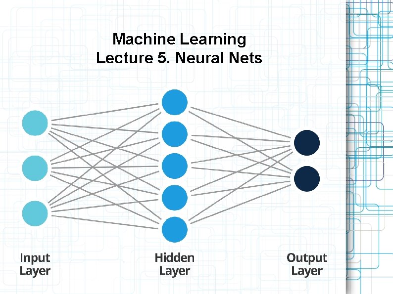
Machine Learning Lecture 5. Neural Nets

Outline Linear perceptron Stochastic gradient descent method Neural nets structure Back propagation Objective functions for regression, binary/multiclass/multilabel classification Activation functions Neural nets design Convolution layers Deep vs shallow nets Dropout and batch normalization

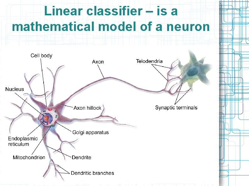
Linear classifier – is a mathematical model of a neuron

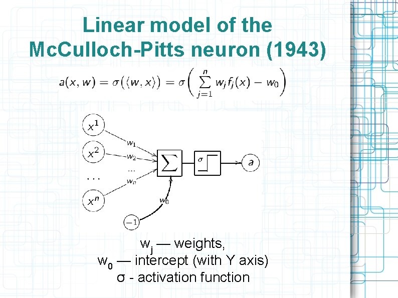
Linear model of the Mc. Culloch-Pitts neuron (1943) wj — weights, w 0 — intercept (with Y axis) σ - activation function

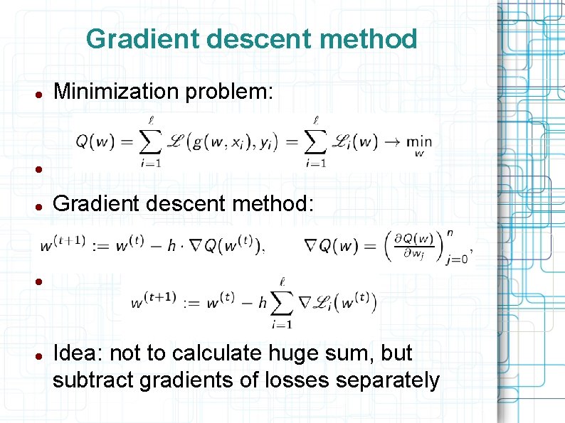
Gradient descent method Minimization problem: Gradient descent method: Idea: not to calculate huge sum, but subtract gradients of losses separately

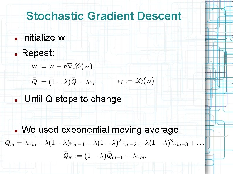
Stochastic Gradient Descent Initialize w Repeat: Until Q stops to change We used exponential moving average:

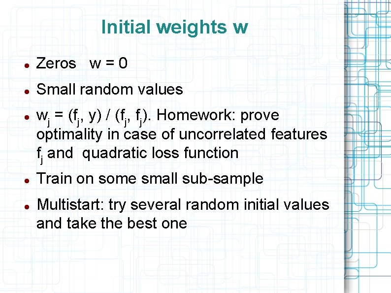
Initial weights w Zeros w = 0 Small random values wj = (fj, y) / (fj, fj). Homework: prove optimality in case of uncorrelated features fj and quadratic loss function Train on some small sub-sample Multistart: try several random initial values and take the best one

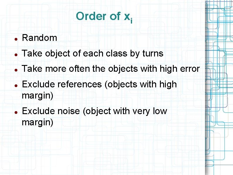
Order of xi Random Take object of each class by turns Take more often the objects with high error Exclude references (objects with high margin) Exclude noise (object with very low margin)

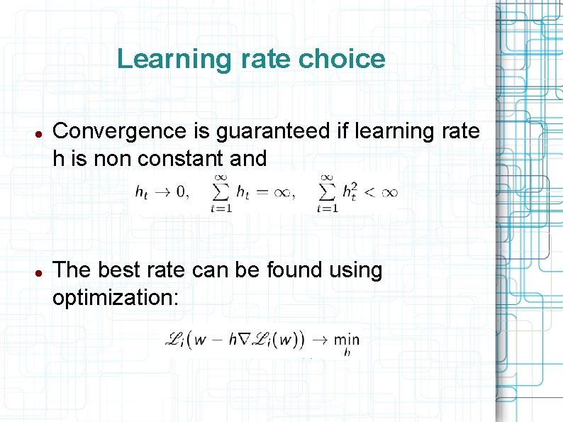
Learning rate choice Convergence is guaranteed if learning rate h is non constant and The best rate can be found using optimization:

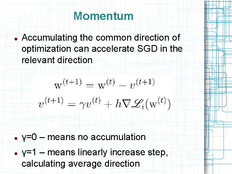
Momentum Accumulating the common direction of optimization can accelerate SGD in the relevant direction γ=0 – means no accumulation γ=1 – means linearly increase step, calculating average direction

Advantages and drawbacks of Stochastic Gradient Descent + Easy to implement + Can optimize any loss functions + Online machine learning (useful when data becomes available in a sequential order) + No need to process the entire sample - Possible slow convergence (or even divergence) - Getting stuck in local minima Overfitting

Overfitting Reasons: Too few objects Too many features Feature multicollinearity Symptoms: Large weights w Instability of predictions Test loss is much greater than train loss Treating: Regularization (weight decay) Early stopping

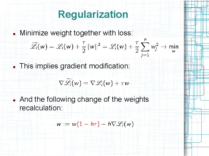
Regularization Minimize weight together with loss: This implies gradient modification: And the following change of the weights recalculation:

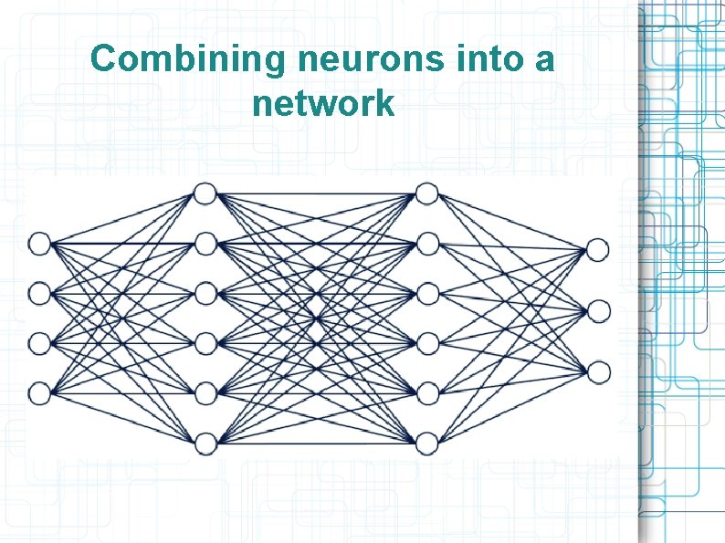
Combining neurons into a network

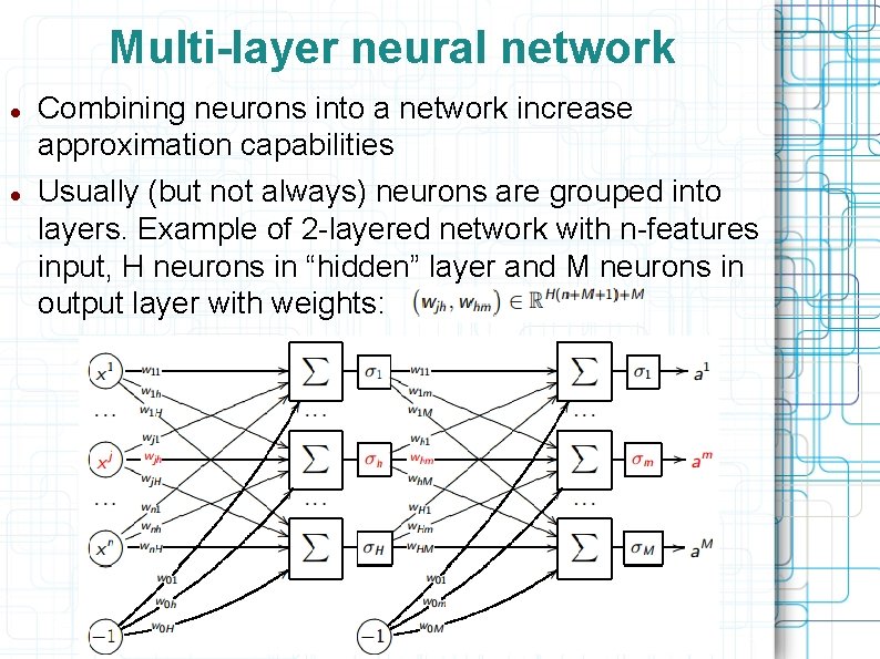
Multi-layer neural network Combining neurons into a network increase approximation capabilities Usually (but not always) neurons are grouped into layers. Example of 2 -layered network with n-features input, H neurons in “hidden” layer and M neurons in output layer with weights:

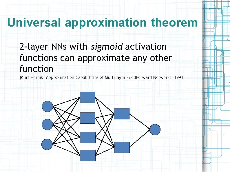
Universal approximation theorem 2 -layer NNs with sigmoid activation functions can approximate any other function (Kurt Hornik: Approximation Capabilities of Multi. Layer Feed. Forward Networks, 1991)

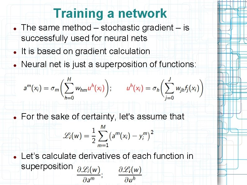
Training a network The same method – stochastic gradient – is successfully used for neural nets It is based on gradient calculation Neural net is just a superposition of functions: For the sake of certainty, let's assume that Let’s calculate derivatives of each function in superposition

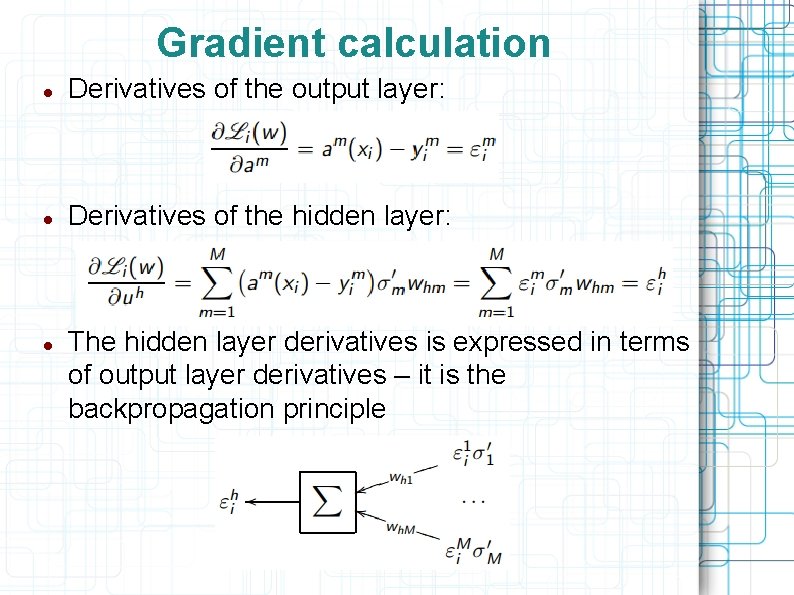
Gradient calculation Derivatives of the output layer: Derivatives of the hidden layer: The hidden layer derivatives is expressed in terms of output layer derivatives – it is the backpropagation principle

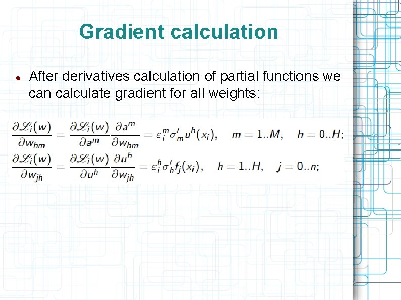
Gradient calculation After derivatives calculation of partial functions we can calculate gradient for all weights:

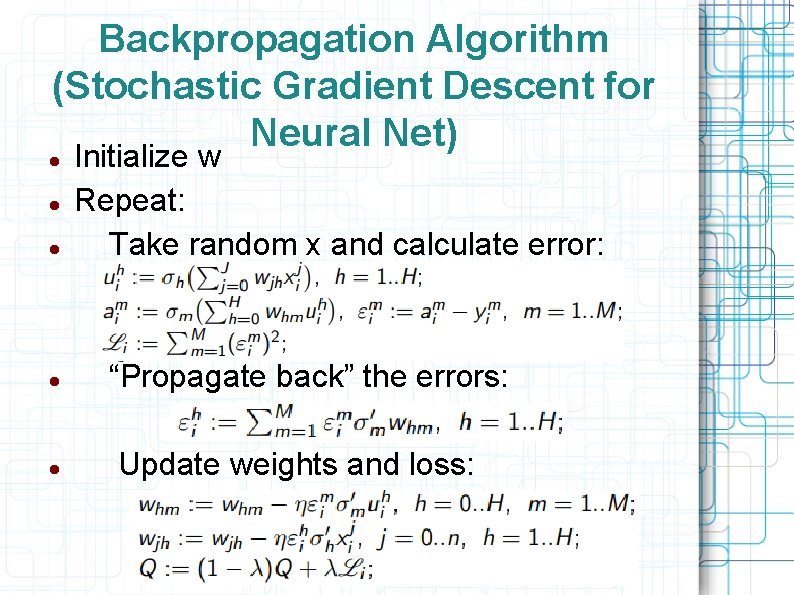
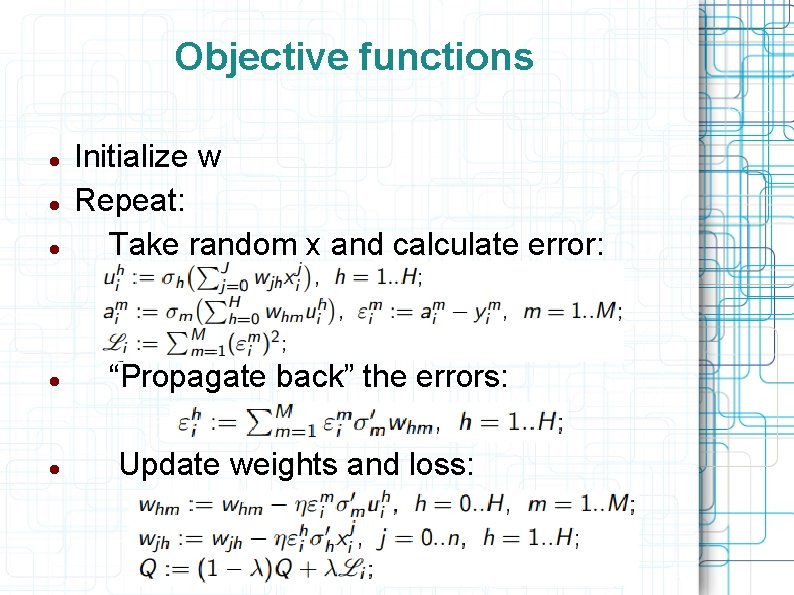
Backpropagation Algorithm (Stochastic Gradient Descent for Neural Net) Initialize w Repeat: Take random x and calculate error: “Propagate back” the errors: Update weights and loss:

Advantages and drawbacks + Fast gradient calculation + Can optimize any loss functions + Online machine learning (useful when data becomes available in a sequential order) + No need to process the entire sample + Can run in parallel - Possible slow convergence (or even divergence) Getting stuck in local minima Overfitting You must have a good experience to choose heuristics correctly

Heuristics Standard (for one neuron): Weight initialization Order of x Optimization of the learning rate Regularization New (for network): Choosing correct activation for each neuron Configure network structure

Objective functions Initialize w Repeat: Take random x and calculate error: “Propagate back” the errors: Update weights and loss:

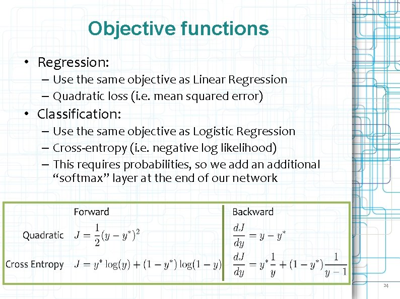
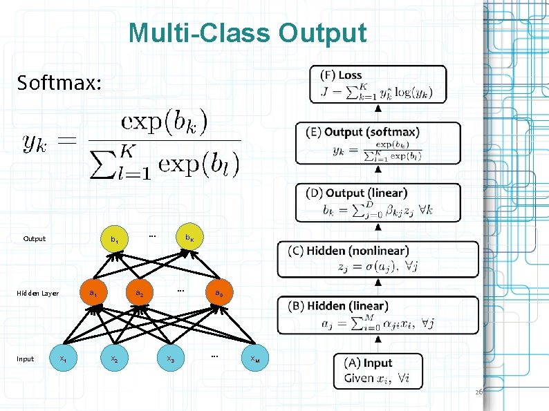
Objective functions • Regression: – Use the same objective as Linear Regression – Quadratic loss (i. e. mean squared error) • Classification: – Use the same objective as Logistic Regression – Cross-entropy (i. e. negative log likelihood) – This requires probabilities, so we add an additional “softmax” layer at the end of our network 24

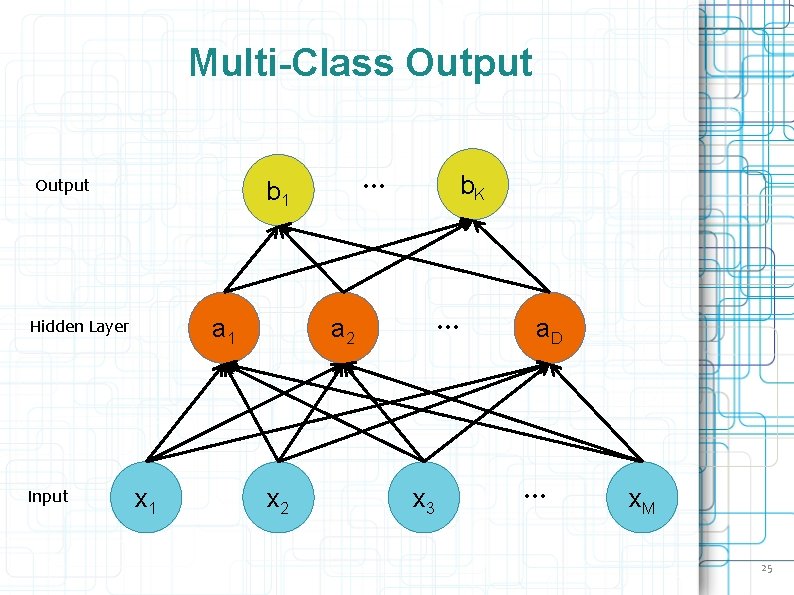
Multi-Class Output a 1 Hidden Layer Input … b 1 x 1 b. K … a 2 x 3 a. D … x. M 25

Multi-Class Output Softmax: Output a 1 Hidden Layer Input … b 1 x 1 b. K … a 2 x 3 a. D … x. M 26

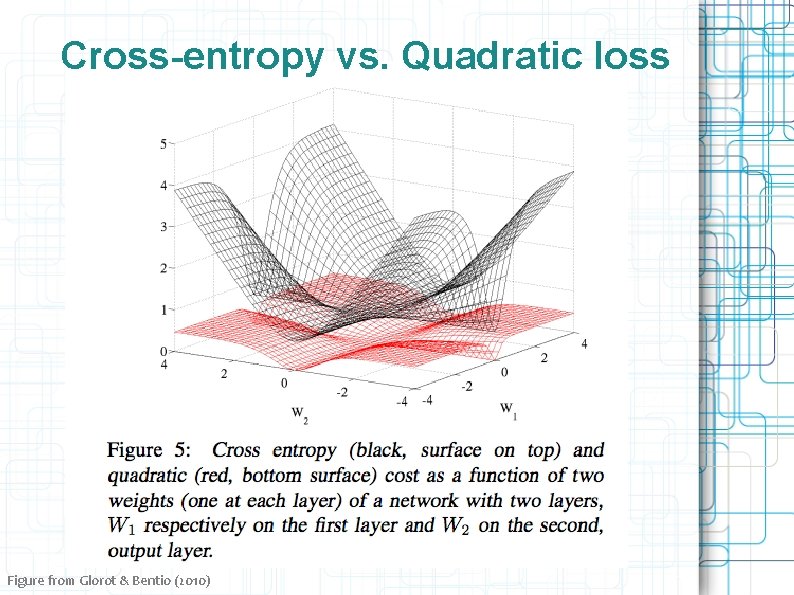
Cross-entropy vs. Quadratic loss Figure from Glorot & Bentio (2010)

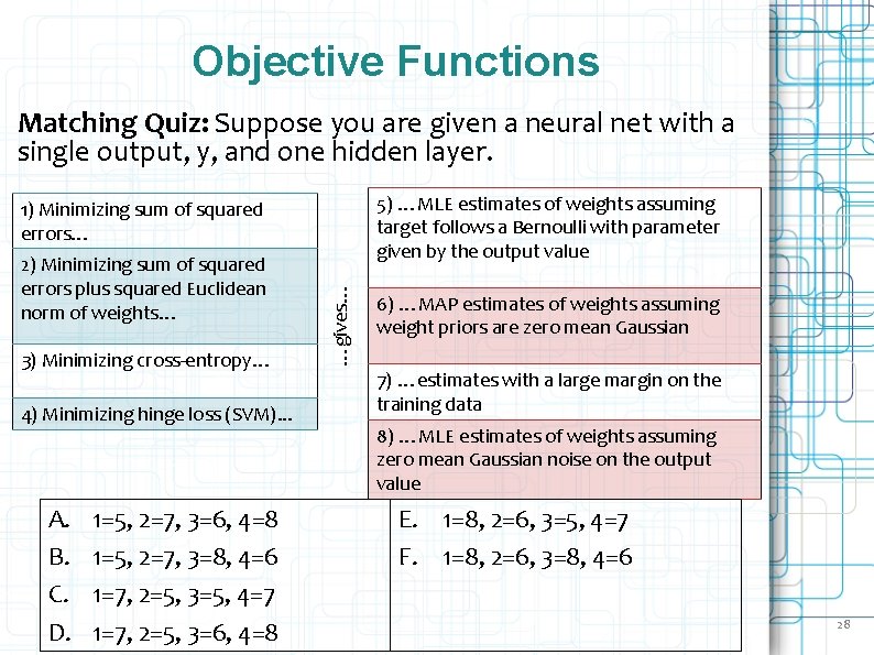
Objective Functions Matching Quiz: Suppose you are given a neural net with a single output, y, and one hidden layer. 5) …MLE estimates of weights assuming target follows a Bernoulli with parameter given by the output value 2) Minimizing sum of squared errors plus squared Euclidean norm of weights… 3) Minimizing cross-entropy… 4) Minimizing hinge loss (SVM). . . A. B. C. D. 1=5, 2=7, 3=6, 4=8 1=5, 2=7, 3=8, 4=6 1=7, 2=5, 3=5, 4=7 1=7, 2=5, 3=6, 4=8 …gives… 1) Minimizing sum of squared errors… 6) …MAP estimates of weights assuming weight priors are zero mean Gaussian 7) …estimates with a large margin on the training data 8) …MLE estimates of weights assuming zero mean Gaussian noise on the output value E. 1=8, 2=6, 3=5, 4=7 F. 1=8, 2=6, 3=8, 4=6 28

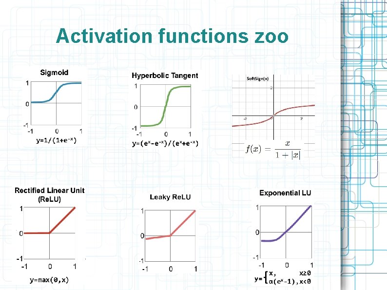
Activation functions zoo

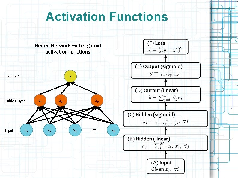
Activation Functions Neural Network with sigmoid activation functions Output y z 1 Hidden Layer Input x 1 … z 2 x 3 z. D … x. M 30

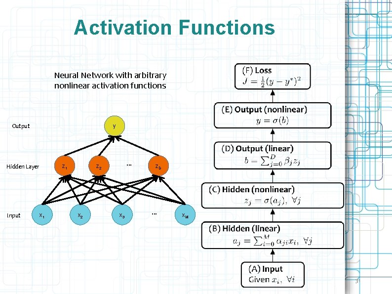
Activation Functions Neural Network with arbitrary nonlinear activation functions Output y z 1 Hidden Layer Input x 1 … z 2 x 3 z. D … x. M 31

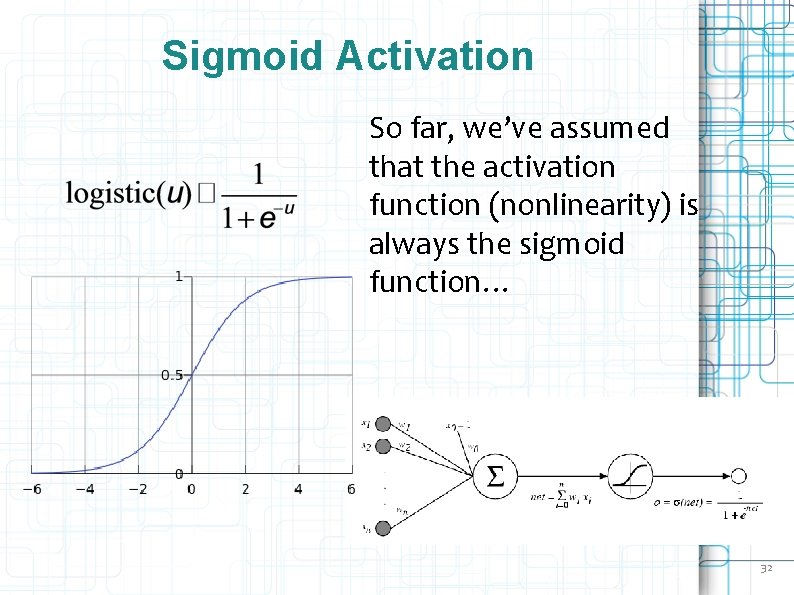
Sigmoid Activation So far, we’ve assumed that the activation function (nonlinearity) is always the sigmoid function… 32

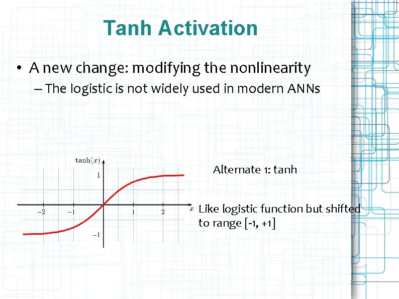
Tanh Activation • A new change: modifying the nonlinearity – The logistic is not widely used in modern ANNs Alternate 1: tanh Like logistic function but shifted to range [-1, +1]

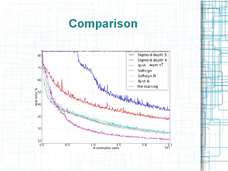
Comparison

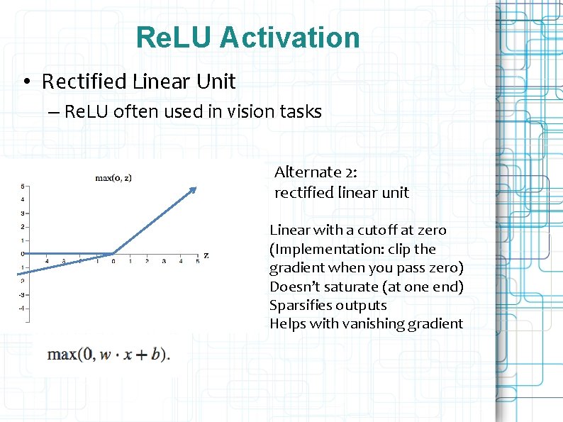
Re. LU Activation • Rectified Linear Unit – Re. LU often used in vision tasks Alternate 2: rectified linear unit Linear with a cutoff at zero (Implementation: clip the gradient when you pass zero) Doesn’t saturate (at one end) Sparsifies outputs Helps with vanishing gradient

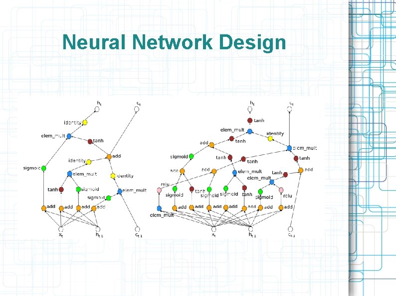
Neural Network Design

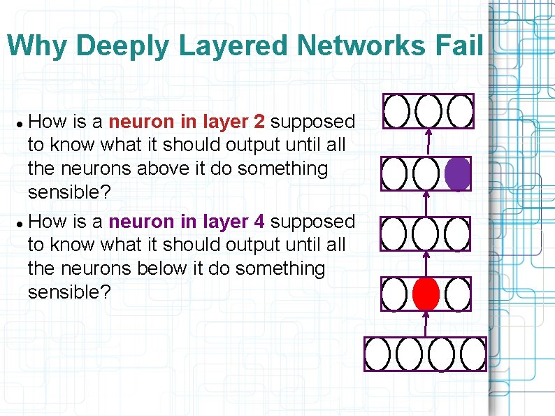
Why Deeply Layered Networks Fail How is a neuron in layer 2 supposed to know what it should output until all the neurons above it do something sensible? How is a neuron in layer 4 supposed to know what it should output until all the neurons below it do something sensible?

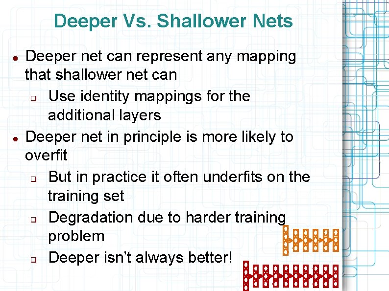
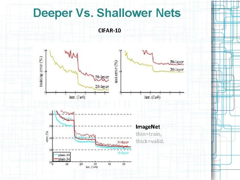
Deeper Vs. Shallower Nets Deeper net can represent any mapping that shallower net can q Use identity mappings for the additional layers Deeper net in principle is more likely to overfit q But in practice it often underfits on the training set q Degradation due to harder training problem q Deeper isn’t always better!

Deeper Vs. Shallower Nets CIFAR-10 Image. Net thin=train, thick=valid.

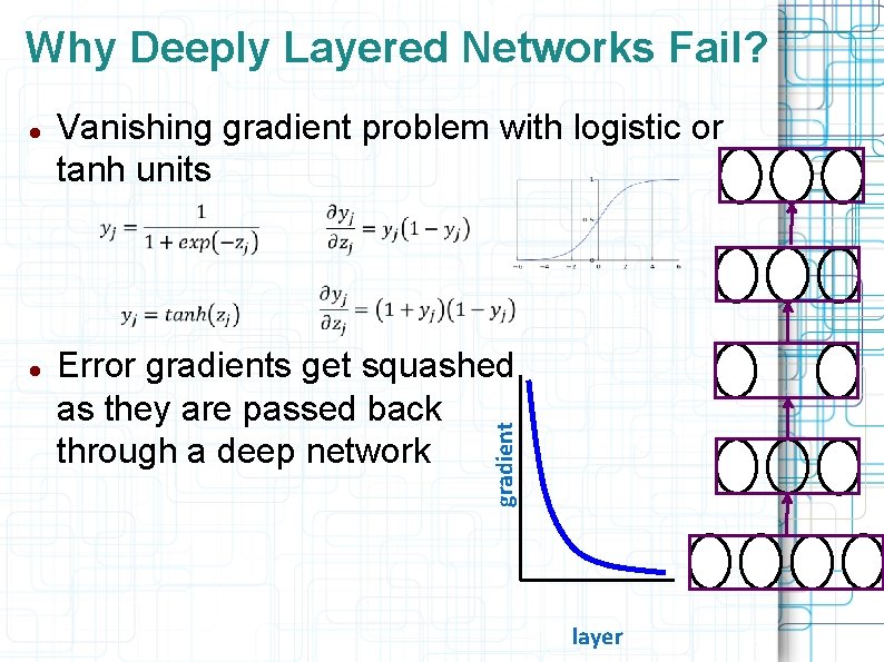
Why Deeply Layered Networks Fail? Vanishing gradient problem with logistic or tanh units Error gradients get squashed as they are passed back through a deep network gradient layer

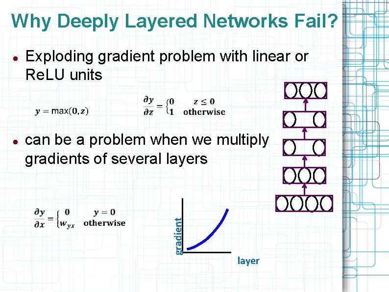
Why Deeply Layered Networks Fail? Exploding gradient problem with linear or Re. LU units can be a problem when we multiply gradients of several layers gradient layer

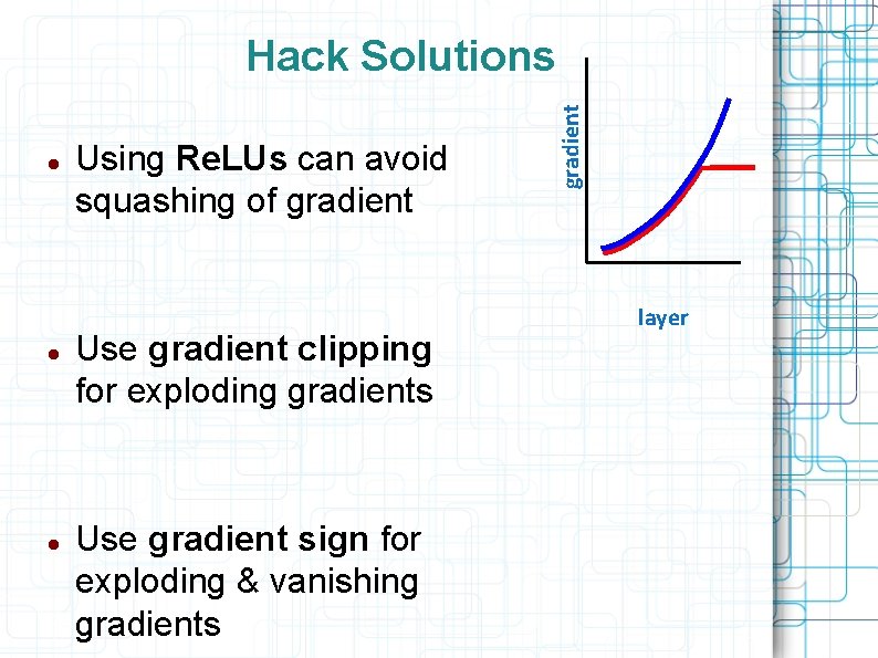
Using Re. LUs can avoid squashing of gradient Use gradient clipping for exploding gradients Use gradient sign for exploding & vanishing gradients gradient Hack Solutions layer

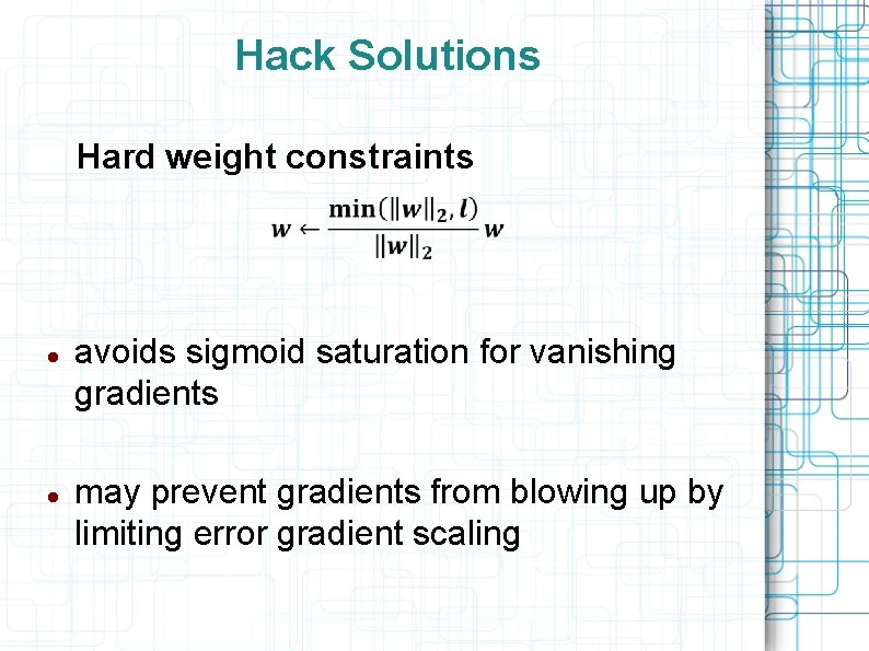
Hack Solutions Hard weight constraints avoids sigmoid saturation for vanishing gradients may prevent gradients from blowing up by limiting error gradient scaling

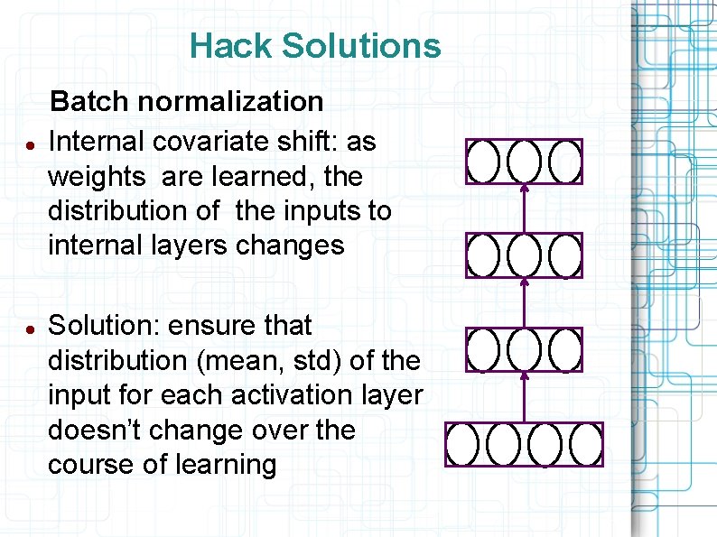
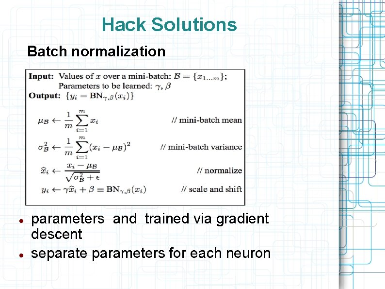
Hack Solutions Batch normalization Internal covariate shift: as weights are learned, the distribution of the inputs to internal layers changes Solution: ensure that distribution (mean, std) of the input for each activation layer doesn’t change over the course of learning

Hack Solutions Batch normalization parameters and trained via gradient descent separate parameters for each neuron

Hack Solutions Unsupervised layer-by-layer pretraining Goal is to start weights off in a sensible configuration instead of using random initial weights Methods of pretraining: q autoencoders q restricted Boltzmann machines The dominant paradigm from ~ 2000 -2010 Still useful today if q not much labeled data q lots of unlabeled data

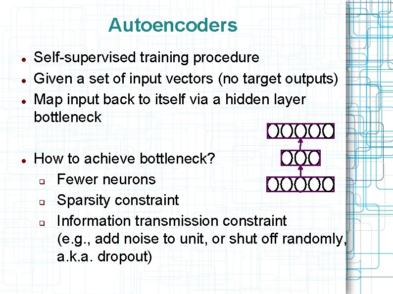
Autoencoders Self-supervised training procedure Given a set of input vectors (no target outputs) Map input back to itself via a hidden layer bottleneck How to achieve bottleneck? q Fewer neurons q Sparsity constraint q Information transmission constraint (e. g. , add noise to unit, or shut off randomly, a. k. a. dropout)

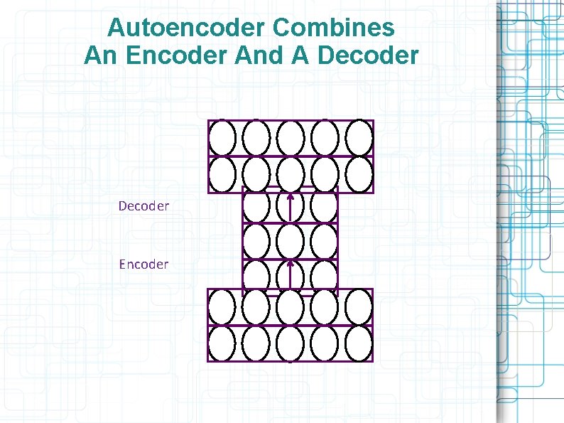
Autoencoder Combines An Encoder And A Decoder Encoder

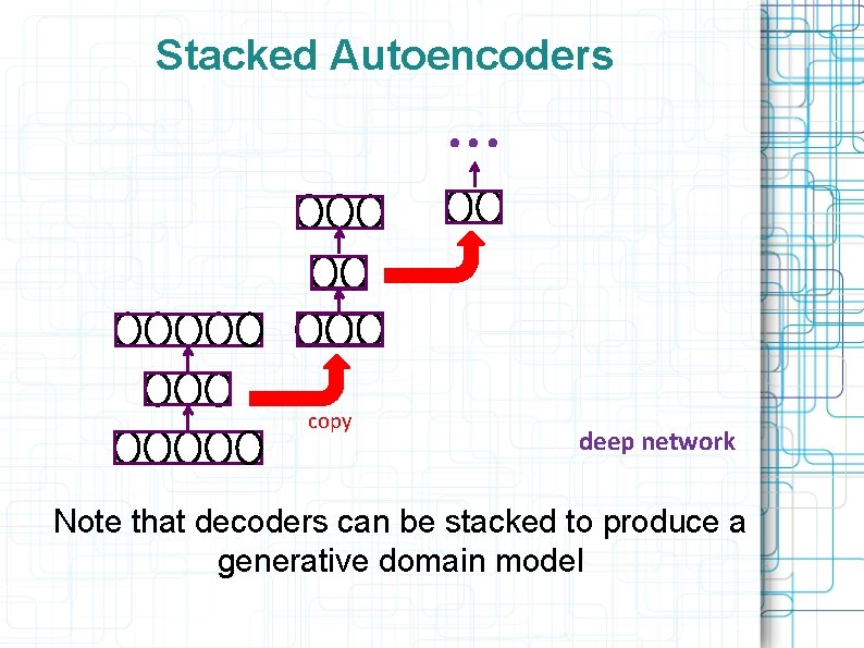
Stacked Autoencoders . . . copy deep network Note that decoders can be stacked to produce a generative domain model

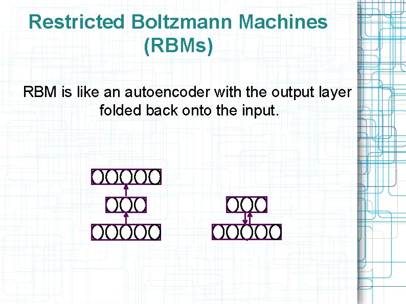
Restricted Boltzmann Machines (RBMs) RBM is like an autoencoder with the output layer folded back onto the input.

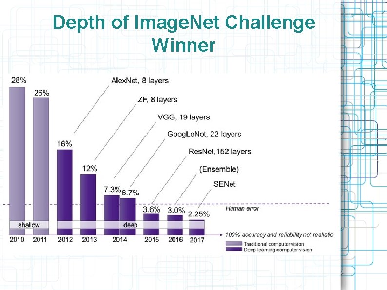
Depth of Image. Net Challenge Winner

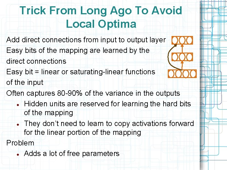
Trick From Long Ago To Avoid Local Optima Add direct connections from input to output layer Easy bits of the mapping are learned by the direct connections Easy bit = linear or saturating-linear functions of the input Often captures 80 -90% of the variance in the outputs Hidden units are reserved for learning the hard bits of the mapping They don’t need to learn to copy activations forward for the linear portion of the mapping Problem Adds a lot of free parameters

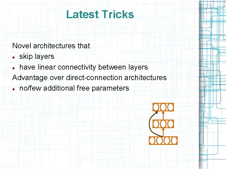
Latest Tricks Novel architectures that skip layers have linear connectivity between layers Advantage over direct-connection architectures no/few additional free parameters

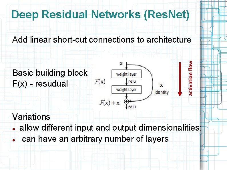
Deep Residual Networks (Res. Net) Basic building block F(x) - resudual activation flow Add linear short-cut connections to architecture Variations allow different input and output dimensionalities: can have an arbitrary number of layers

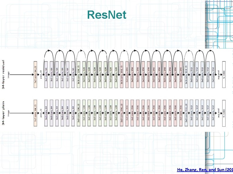
Res. Net He, Zhang, Ren, and Sun (201

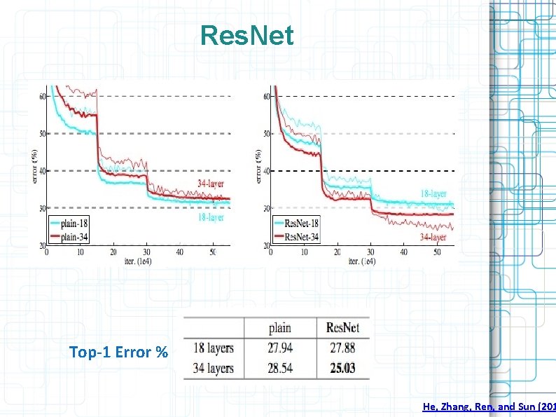
Res. Net Top-1 Error % He, Zhang, Ren, and Sun (201

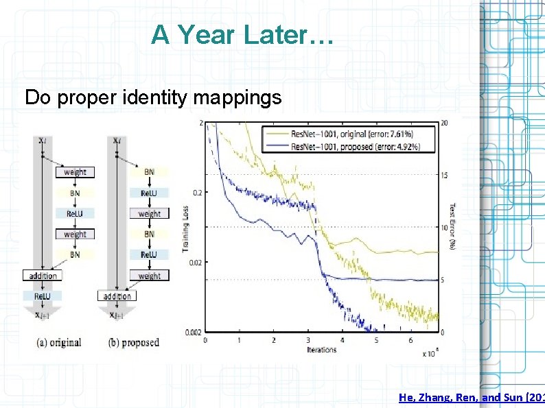
A Year Later… Do proper identity mappings He, Zhang, Ren, and Sun (201

Highway Networks Suppose each layer of the network made a decision whether to copy input forward perform a nonlinear transform of the input Weighting coefficient Coefficient is a function of the input Srivastava, Greff, & Schmidhuber (2015)

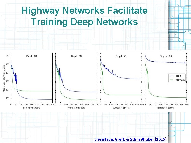
Highway Networks Facilitate Training Deep Networks Srivastava, Greff, & Schmidhuber (2015)

Generative networks Producing images by network is used in various applications: Improving image quality (resolution, denoising, reconstruction) Changing image controlled by voice angle, smile degree, expression, light, color… other image (fake videos) Generating real images from scratch Style transfer

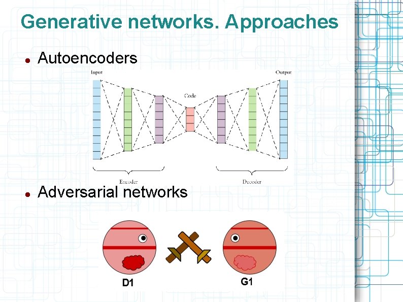
Generative networks. Approaches Autoencoders Adversarial networks

Generative networks Producing images by network is used in various applications: Improving image quality (resolution, denoising, reconstruction) Changing image controlled by voice angle, smile degree, expression, light, color… other image (fake videos) Generating real images from scratch Style transfer

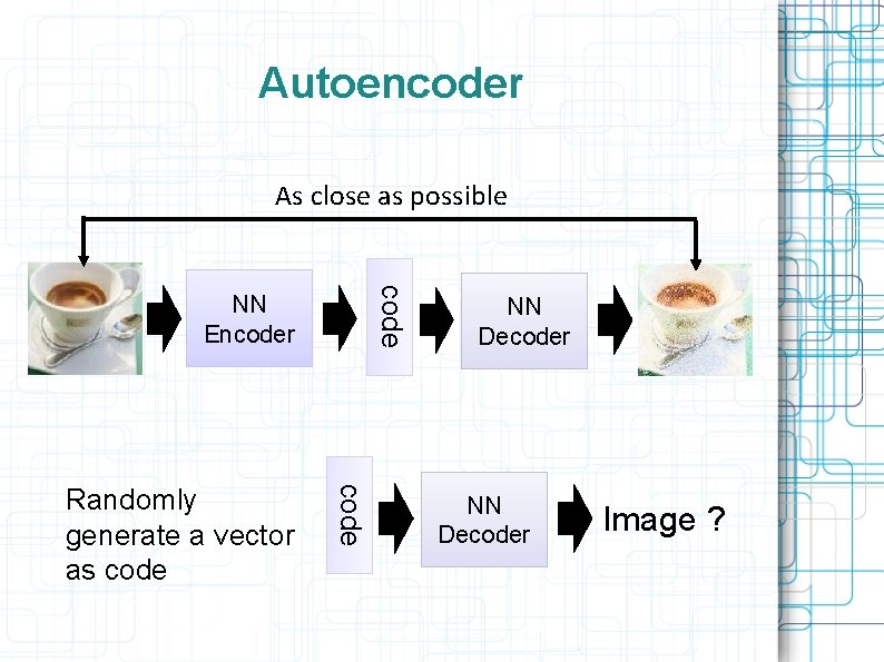
Autoencoder As close as possible code NN Encoder code Randomly generate a vector as code NN Decoder Image ?

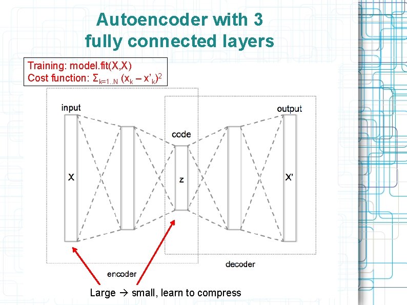
Autoencoder with 3 fully connected layers Training: model. fit(X, X) Cost function: Σk=1. . N (xk – x’k)2 Large small, learn to compress

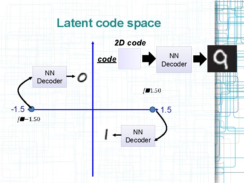
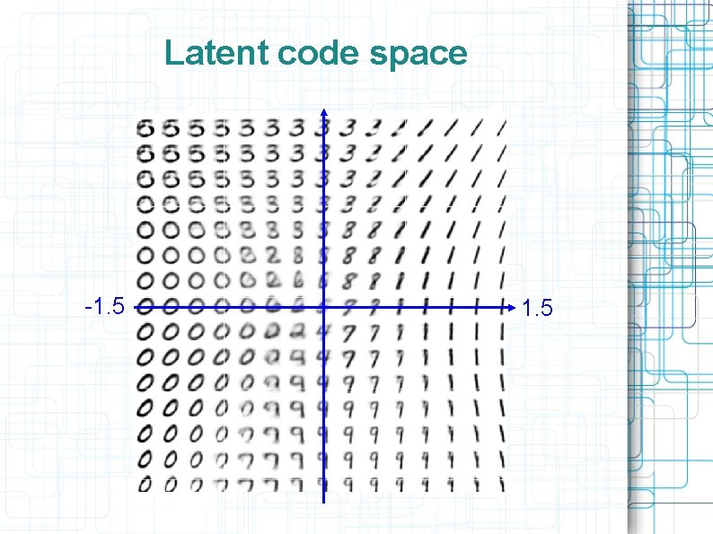
Latent code space 2 D code NN Decoder -1. 5 NN Decoder

Latent code space -1. 5

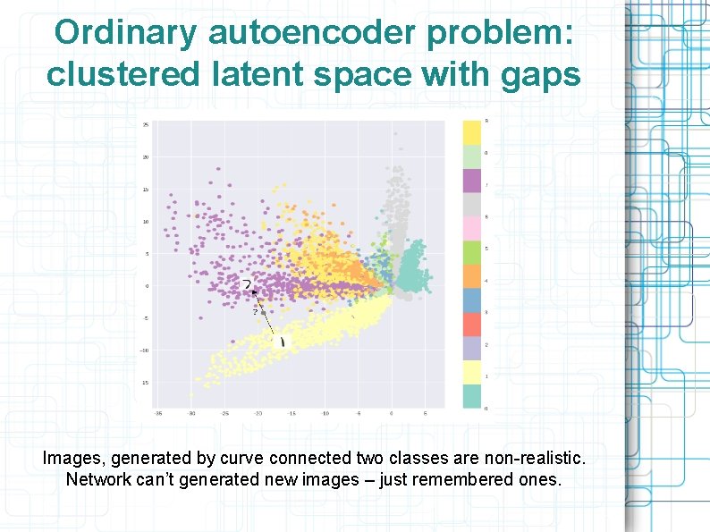
Ordinary autoencoder problem: clustered latent space with gaps Images, generated by curve connected two classes are non-realistic. Network can’t generated new images – just remembered ones.

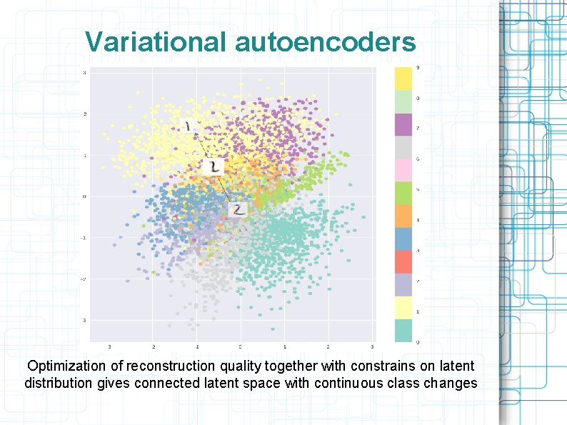
Variational autoencoders Optimization of reconstruction quality together with constrains on latent distribution gives connected latent space with continuous class changes

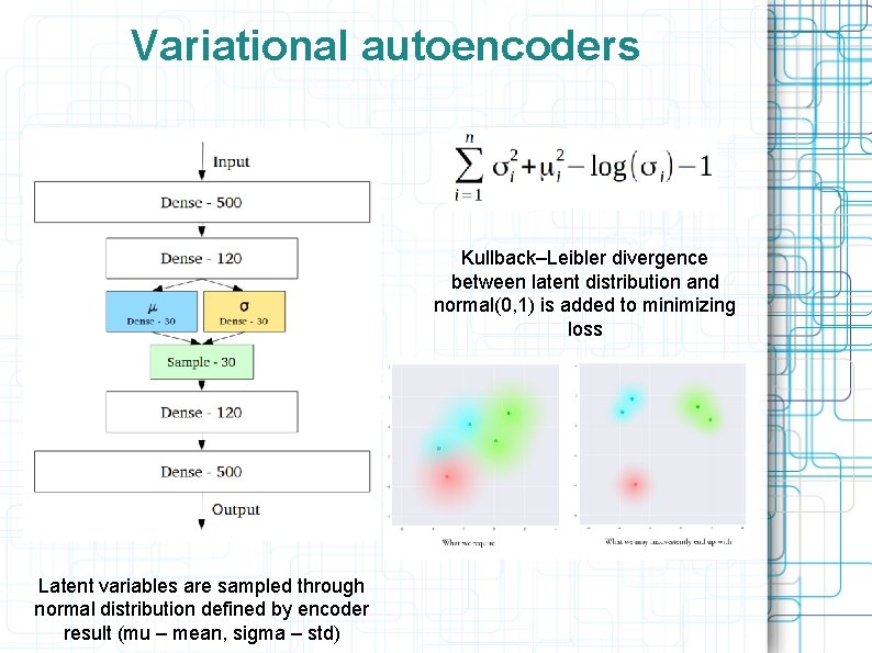
Variational autoencoders Kullback–Leibler divergence between latent distribution and normal(0, 1) is added to minimizing loss Latent variables are sampled through normal distribution defined by encoder result (mu – mean, sigma – std)

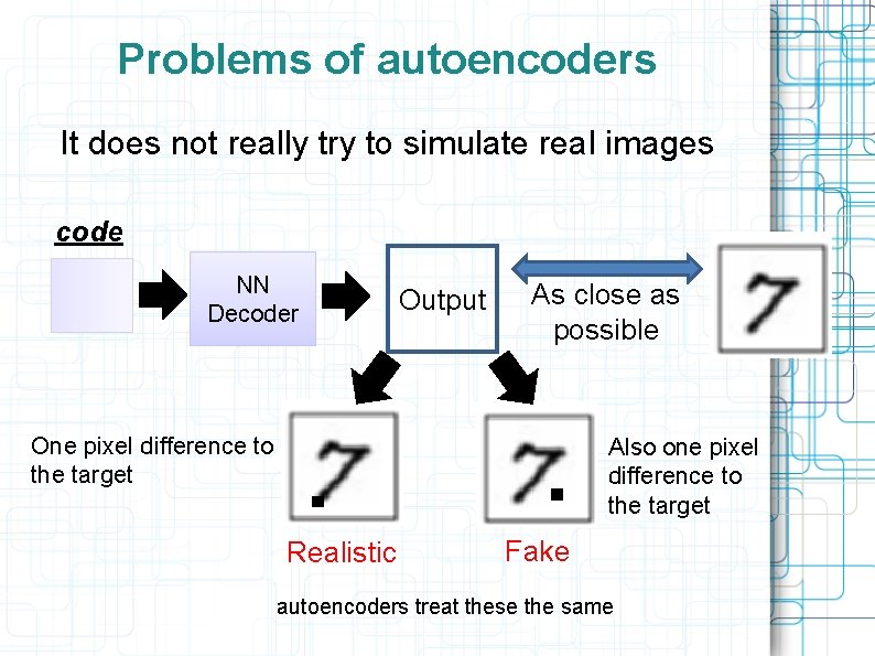
Problems of autoencoders It does not really try to simulate real images code NN Decoder Output As close as possible One pixel difference to the target Also one pixel difference to the target Realistic Fake autoencoders treat these the same

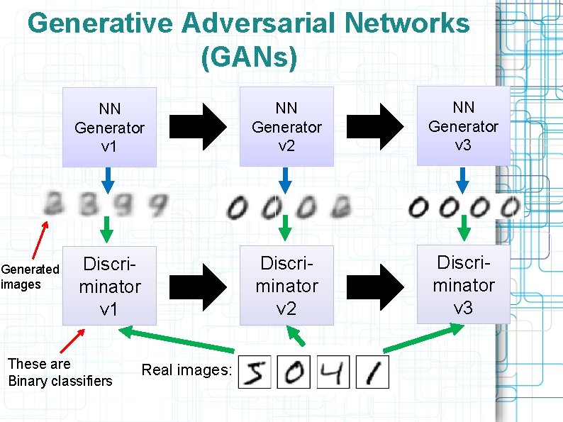
Generative Adversarial Networks (GANs) Generated images NN Generator v 1 NN Generator v 2 NN Generator v 3 Discriminator v 1 Discriminator v 2 Discriminator v 3 These are Binary classifiers Real images:

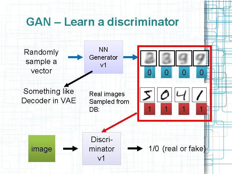
GAN – Learn a discriminator Randomly sample a vector Something like Decoder in VAE image NN Generator v 1 Real images Sampled from DB: Discriminator v 1 0 0 1 1 1/0 (real or fake)

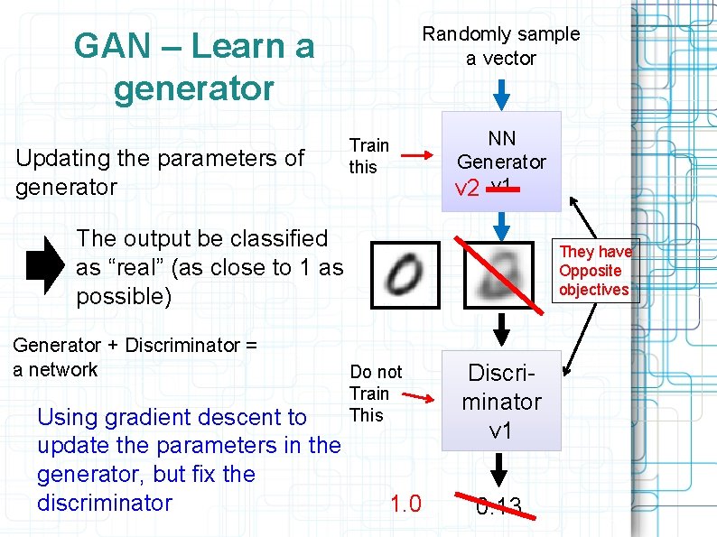
Randomly sample a vector GAN – Learn a generator Updating the parameters of generator Train this NN Generator v 2 v 1 The output be classified as “real” (as close to 1 as possible) Generator + Discriminator = a network Using gradient descent to update the parameters in the generator, but fix the discriminator They have Opposite objectives Do not Train This 1. 0 Discriminator v 1 0. 13