Machine learning Lecture 4 Linear algorithms Outline Linear

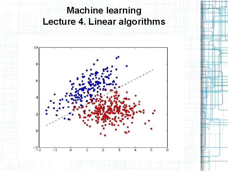
Machine learning Lecture 4. Linear algorithms

Outline Linear regression Classification: Logistic regression (probability-based) Related topics: One hot encoding and ROC SVM (geometry-based) Linear perceptron (biology-based) – next lecture about NN

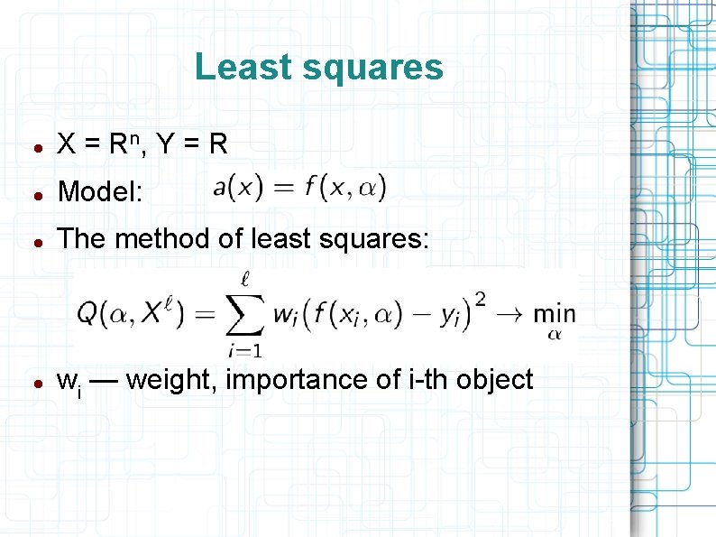
Least squares X = Rn, Y = R Model: The method of least squares: wi — weight, importance of i-th object

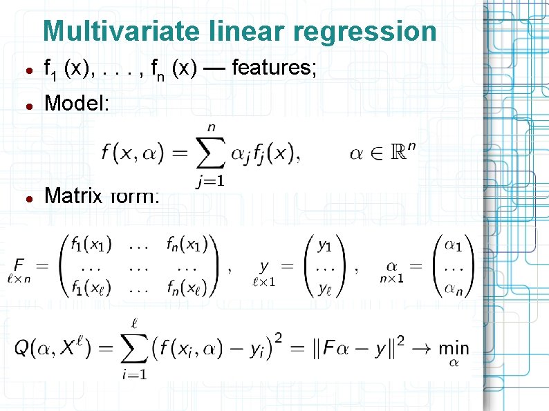
Multivariate linear regression f 1 (x), . . . , fn (x) — features; Model: Matrix form:

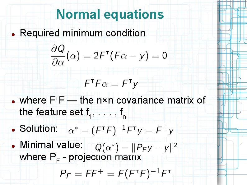
Normal equations Required minimum condition where Fт. F — the n×n covariance matrix of the feature set f 1, . . . , fn Solution: Minimal value: where PF - projection matrix

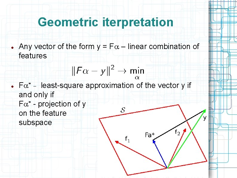
Geometric iterpretation Any vector of the form y = Fa – linear combination of features Fa* _ least-square approximation of the vector y if and only if Fa* - projection of y on the feature subspace

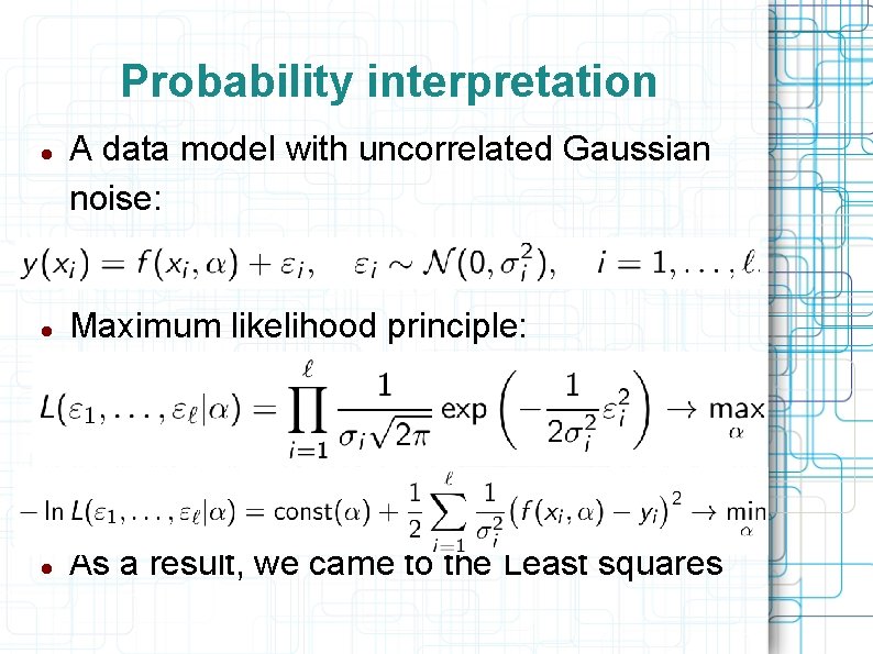
Probability interpretation A data model with uncorrelated Gaussian noise: Maximum likelihood principle: As a result, we came to the Least squares

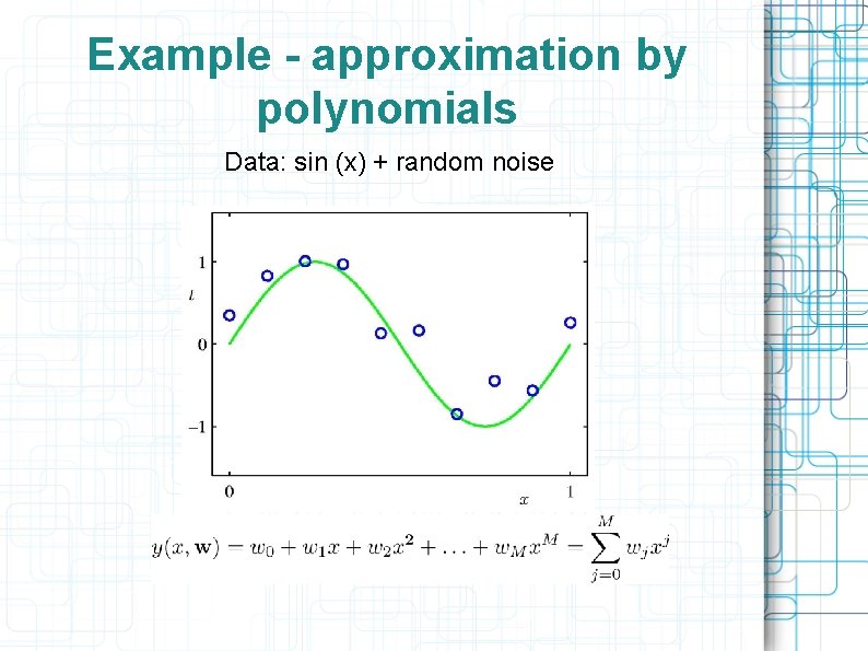
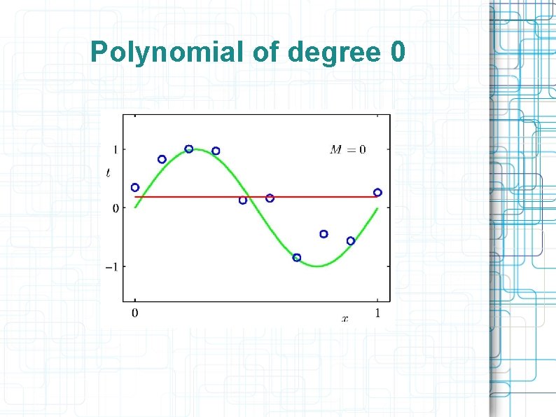
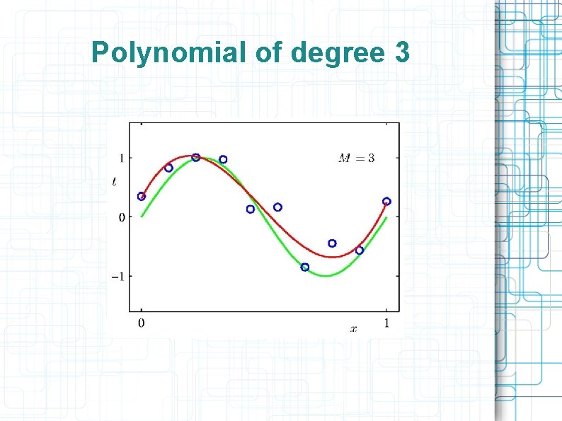
Example - approximation by polynomials Data: sin (x) + random noise

Polynomial of degree 0

Polynomial of degree 3

Polynomial of degree 9

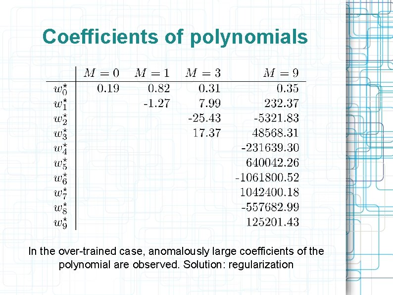
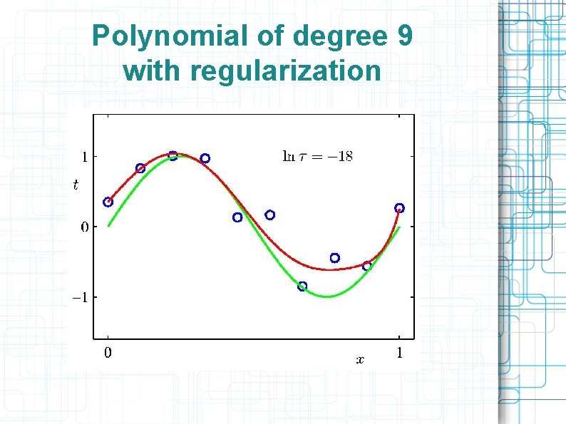
Coefficients of polynomials In the over-trained case, anomalously large coefficients of the polynomial are observed. Solution: regularization

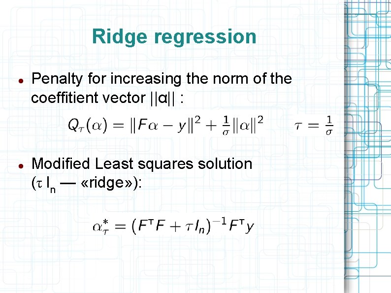
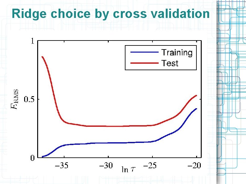
Ridge regression Penalty for increasing the norm of the coeffitient vector ||α|| : Modified Least squares solution (τ In — «ridge» ):

Polynomial of degree 9 with regularization

Ridge choice by cross validation

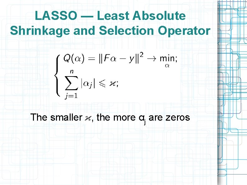
LASSO — Least Absolute Shrinkage and Selection Operator The smaller κ, the more αj are zeros

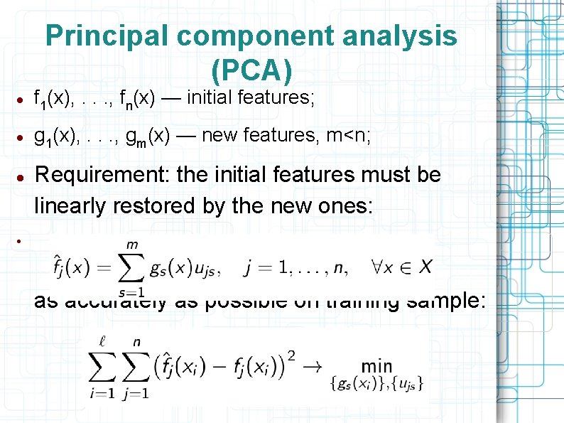
Principal component analysis (PCA) f 1(x), . . . , fn(x) — initial features; g 1(x), . . . , gm(x) — new features, m<n; Requirement: the initial features must be linearly restored by the new ones: as accurately as possible on training sample:

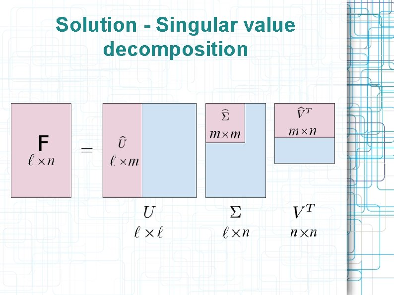
Solution - Singular value decomposition

SVD application for image compression m=10 m=30 m=100

How many primary components to use? The "steep slope" criterion:

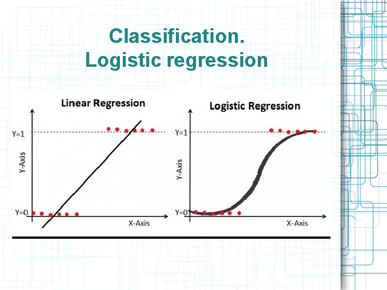
Classification. Logistic regression

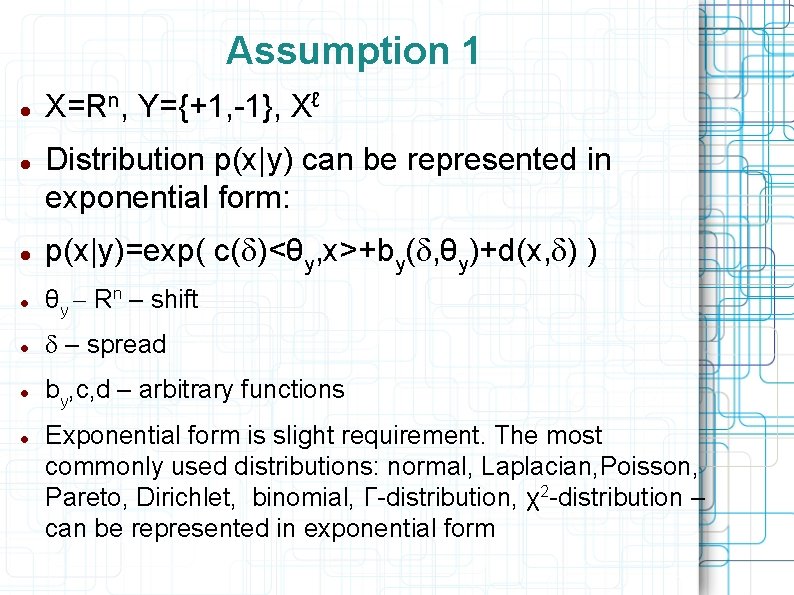
Assumption 1 X=Rn, Y={+1, -1}, Xℓ Distribution p(x|y) can be represented in exponential form: p(x|y)=exp( c(d)<θy, x>+by(d, θy)+d(x, d) ) θy - Rn – shift d – spread by, c, d – arbitrary functions Exponential form is slight requirement. The most commonly used distributions: normal, Laplacian, Poisson, Pareto, Dirichlet, binomial, Γ-distribution, χ2 -distribution – can be represented in exponential form

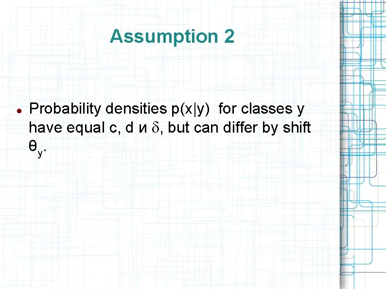
Assumption 2 Probability densities p(x|y) for classes y have equal c, d и d, but can differ by shift θy.

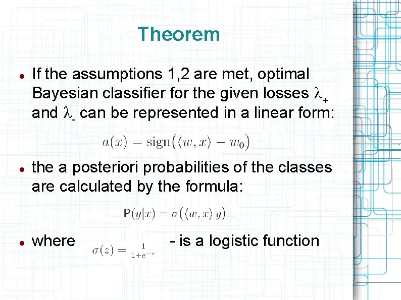
Theorem If the assumptions 1, 2 are met, optimal Bayesian classifier for the given losses l+ and l- can be represented in a linear form: the a posteriori probabilities of the classes are calculated by the formula: where - is a logistic function

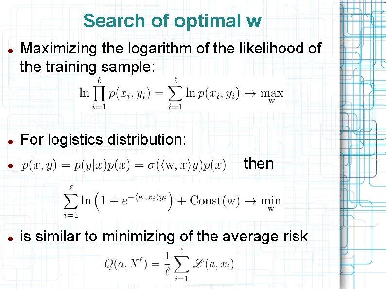
Search of optimal w Maximizing the logarithm of the likelihood of the training sample: For logistics distribution: then is similar to minimizing of the average risk

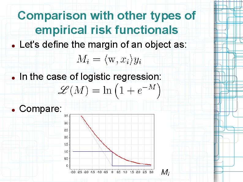
Comparison with other types of empirical risk functionals Let's define the margin of an object as: In the case of logistic regression: Compare:

One Hot encoding Let x be the only feature (polynominal, encoded by: 0, 1, 2, . . . k) Classifier: a(x) = sign(wx+w 0) Difficulty: we can’t choose weight w so that the classifier was not monotonous. For all possible w and w 0 a(x) > 0 when x > w 0/w and a(x) ≤ 0 otherwise

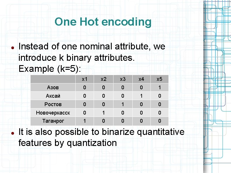
One Hot encoding Instead of one nominal attribute, we introduce k binary attributes. Example (k=5): x 1 x 2 x 3 x 4 x 5 Азов 0 0 1 Аксай 0 0 0 1 0 Ростов 0 0 1 0 0 Новочеркасск 0 1 0 0 0 Таганрог 1 0 0 It is also possible to binarize quantitative features by quantization

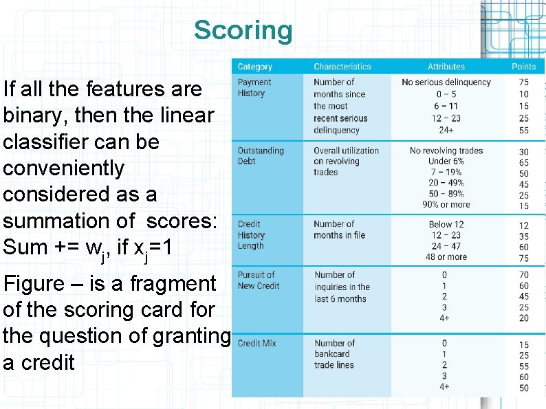
Scoring If all the features are binary, then the linear classifier can be conveniently considered as a summation of scores: Sum += wj, if xj=1 Figure – is a fragment of the scoring card for the question of granting a credit

Different losses In applications losses can be revised New optimal classifier has the same w, but different threshold defined by w 0 Optimal accuracy for different losses differs and we can`t compare it Better to use quality measure, which doesn`t depend on losses. Quality of order, given by w

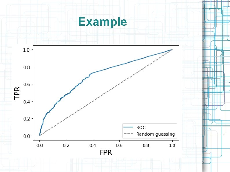
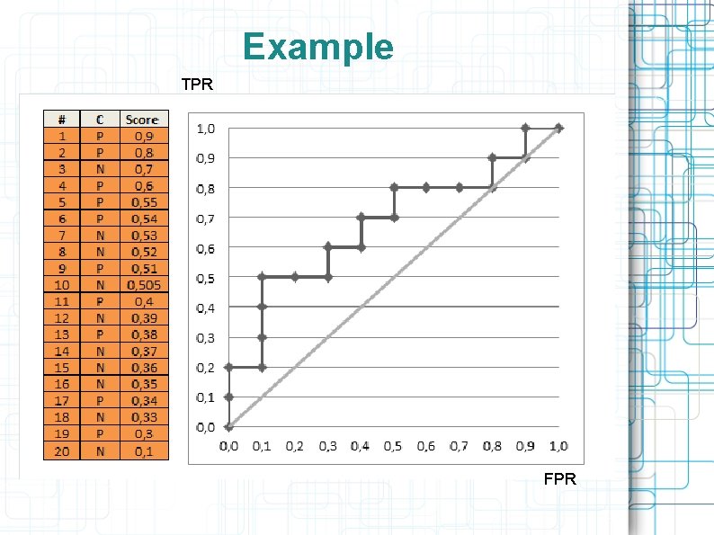
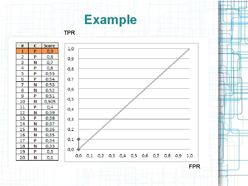
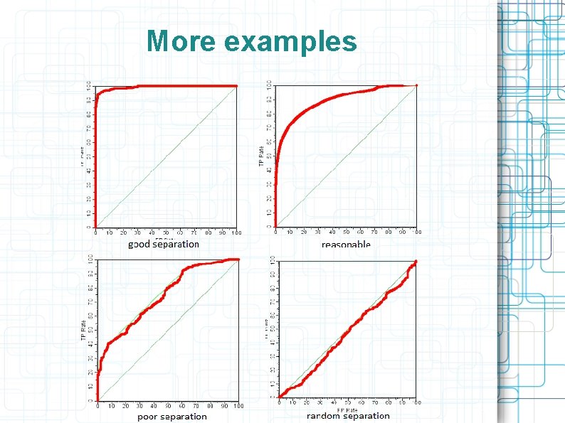
ROC – receiver operating characteristic Each point of the curve corresponds to some threshold (i. e. losses, w 0) X axis: FPR (false positive rate) – ratio of objects with y=-1 and a(x)=+1 among y=-1 Y axis: TPR (true positive rate) – ratio of objects with y=+1 and a(x)=+1 among y=+1

Example

Example TPR FPR

Example TPR FPR

More examples

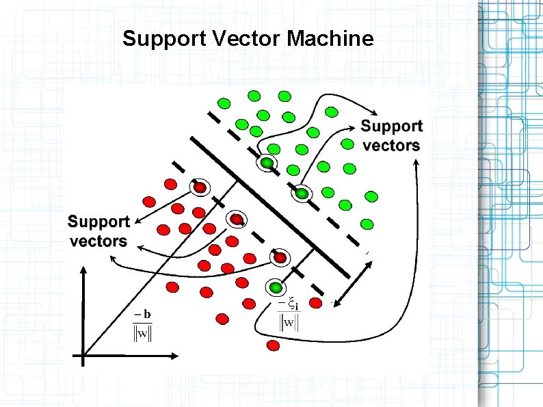
Support Vector Machine

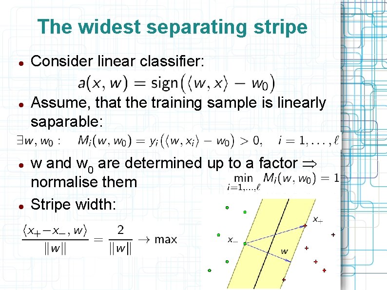
The widest separating stripe Consider linear classifier: Assume, that the training sample is linearly saparable: w and w 0 are determined up to a factor Þ normalise them Stripe width:

Support vector machine for a linearly separable sample What should we do if the sample is not separable by a hyperplane?

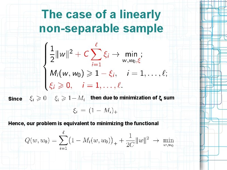
The case of a linearly non-separable sample Since then due to minimization of xi sum Hence, our problem is equivalent to minimizing the functional

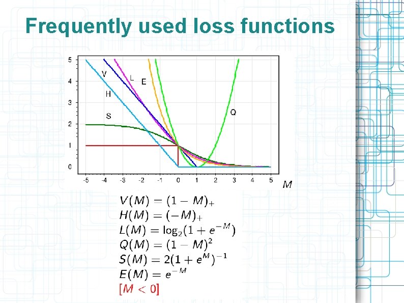
Frequently used loss functions