Machine Learning Graphical Models Eric Xing Lecture 12

Machine Learning Graphical Models Eric Xing Lecture 12, August 14, 2010 Reading: Eric Xing © Eric Xing @ CMU, 2006 -2010

Inference and Learning l A BN M describes a unique probability distribution P l Typical tasks: l Task 1: How do we answer queries about P? l l l We use inference as a name for the process of computing answers to such queries So far we have learned several algorithms for exact and approx. inference Task 2: How do we estimate a plausible model M from data D? i. We use learning as a name for the process of obtaining point estimate of M. ii. But for Bayesian, they seek p(M |D), which is actually an inference problem. iii. When not all variables are observable, even computing point estimate of M need to do inference to impute the missing data. Eric Xing © Eric Xing @ CMU, 2006 -2010 2

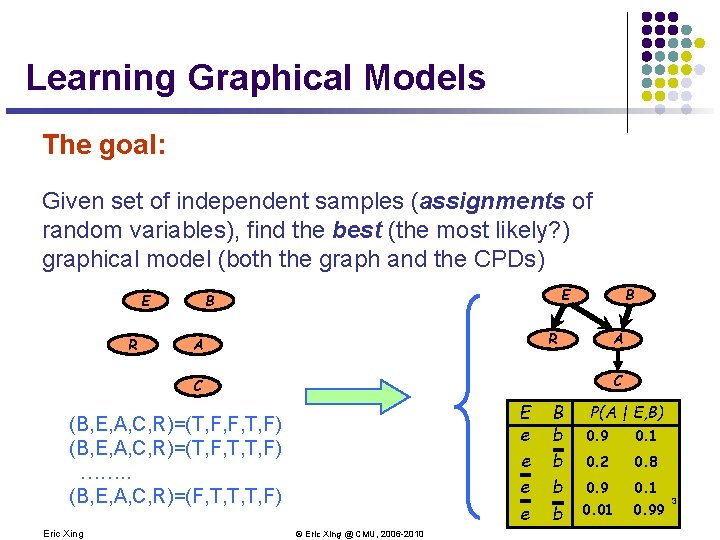
Learning Graphical Models The goal: Given set of independent samples (assignments of random variables), find the best (the most likely? ) graphical model (both the graph and the CPDs) R B E R A A C C E e e (B, E, A, C, R)=(T, F, F, T, F) (B, E, A, C, R)=(T, F, T, T, F) ……. . (B, E, A, C, R)=(F, T, T, T, F) Eric Xing © Eric Xing @ CMU, 2006 -2010 B b b P(A | E, B) 0. 9 0. 1 0. 2 0. 8 0. 9 0. 1 0. 01 0. 99 3

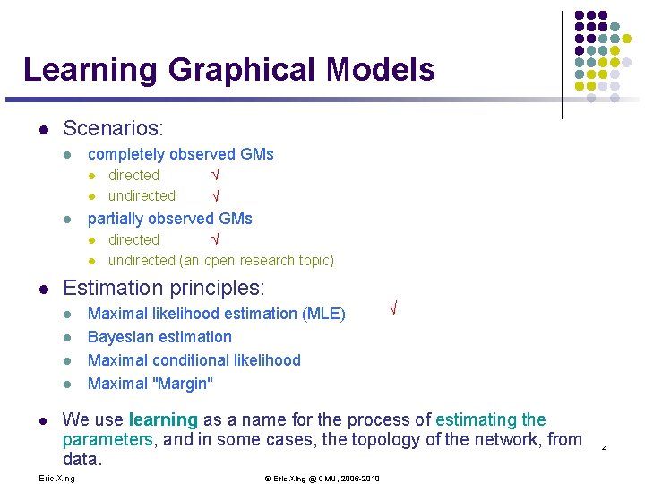
Learning Graphical Models l Scenarios: l l completely observed GMs l directed Ö l undirected Ö partially observed GMs l directed Ö l l Estimation principles: l l l undirected (an open research topic) Maximal likelihood estimation (MLE) Bayesian estimation Maximal conditional likelihood Maximal "Margin" Ö We use learning as a name for the process of estimating the parameters, and in some cases, the topology of the network, from data. Eric Xing © Eric Xing @ CMU, 2006 -2010 4

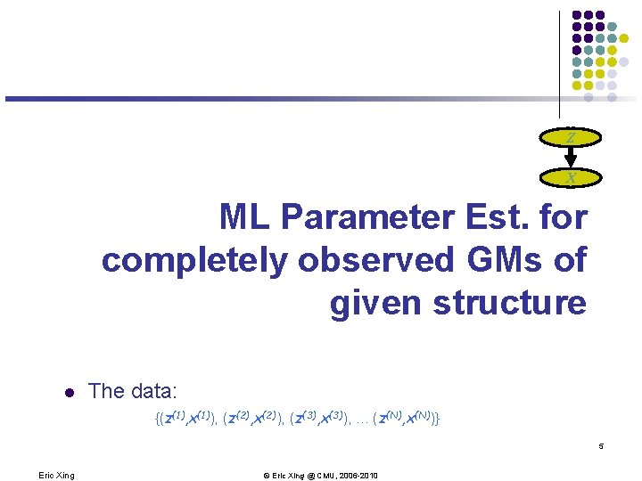
Z X ML Parameter Est. for completely observed GMs of given structure l The data: {(z(1), x(1)), (z(2), x(2)), (z(3), x(3)), . . . (z(N), x(N))} 5 Eric Xing © Eric Xing @ CMU, 2006 -2010

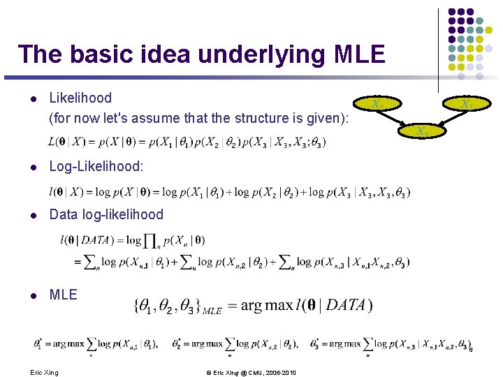
The basic idea underlying MLE l Likelihood (for now let's assume that the structure is given): l Log-Likelihood: l Data log-likelihood l MLE X 1 X 2 X 3 6 Eric Xing © Eric Xing @ CMU, 2006 -2010

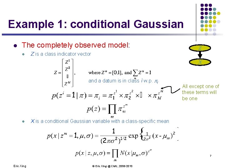
Example 1: conditional Gaussian l The completely observed model: l Z is a class indicator vector Z X and a datum is in class i w. p. pi l All except one of these terms will be one X is a conditional Gaussian variable with a class-specific mean 7 Eric Xing © Eric Xing @ CMU, 2006 -2010

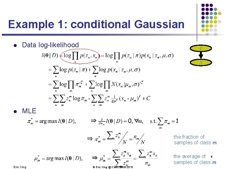
Example 1: conditional Gaussian l Data log-likelihood Z X l MLE the fraction of samples of class m Eric Xing the average of 8 samples of class m © Eric Xing @ CMU, 2006 -2010

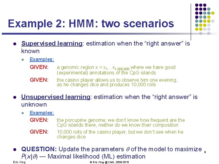
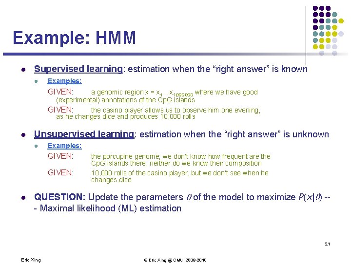
Example 2: HMM: two scenarios l Supervised learning: estimation when the “right answer” is known l Examples: GIVEN: l Unsupervised learning: estimation when the “right answer” is unknown l Examples: GIVEN: l a genomic region x = x 1…x 1, 000 where we have good (experimental) annotations of the Cp. G islands the casino player allows us to observe him one evening, as he changes dice and produces 10, 000 rolls the porcupine genome; we don’t know how frequent are the Cp. G islands there, neither do we know their composition 10, 000 rolls of the casino player, but we don’t see when he changes dice QUESTION: Update the parameters of the model to maximize P(x| ) --- Maximal likelihood (ML) estimation Eric Xing © Eric Xing @ CMU, 2006 -2010 9

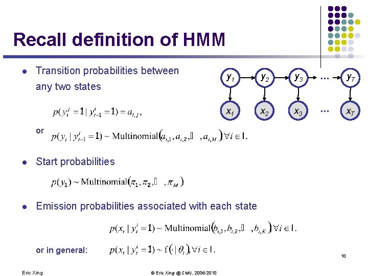
Recall definition of HMM l Transition probabilities between any two states y 1 y 2 y 3 . . . y. T x. A 1 x. A 2 x. A 3 . . . x. AT or l Start probabilities l Emission probabilities associated with each state or in general: Eric Xing 10 © Eric Xing @ CMU, 2006 -2010

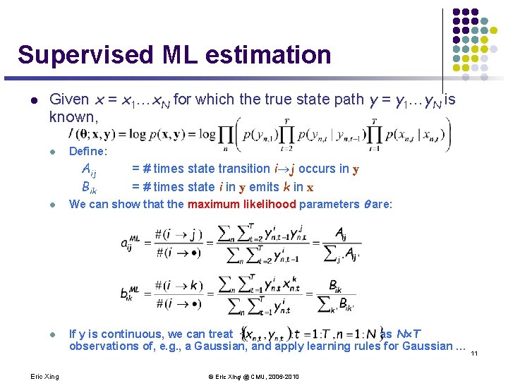
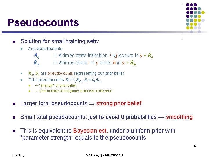
Supervised ML estimation l Given x = x 1…x. N for which the true state path y = y 1…y. N is known, l Define: Aij Bik l l Eric Xing = # times state transition i j occurs in y = # times state i in y emits k in x We can show that the maximum likelihood parameters are: If y is continuous, we can treat as N´T observations of, e. g. , a Gaussian, and apply learning rules for Gaussian … 11 © Eric Xing @ CMU, 2006 -2010

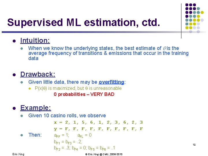
Supervised ML estimation, ctd. l Intuition: l l When we know the underlying states, the best estimate of is the average frequency of transitions & emissions that occur in the training data Drawback: l Given little data, there may be overfitting: l l P(x| ) is maximized, but is unreasonable 0 probabilities – VERY BAD Example: l l Eric Xing Given 10 casino rolls, we observe Then: x = 2, 1, 5, 6, 1, 2, 3, 6, 2, 3 y = F, F, F, F a. FF = 1; a. FL = 0 b. F 1 = b. F 3 =. 2; b. F 2 =. 3; b. F 4 = 0; b. F 5 = b. F 6 =. 1 © Eric Xing @ CMU, 2006 -2010 12

Pseudocounts l Solution for small training sets: l Add pseudocounts Aij Bik = # times state transition i j occurs in y + Rij = # times state i in y emits k in x + Sik l Rij, Sij are pseudocounts representing our prior belief l Total pseudocounts: Ri = Sj. Rij , Si = Sk. Sik , l --- "strength" of prior belief, l --- total number of imaginary instances in the prior l Larger total pseudocounts strong prior belief l Small total pseudocounts: just to avoid 0 probabilities --- smoothing l This is equivalent to Bayesian est. under a uniform prior with "parameter strength" equals to the pseudocounts 13 Eric Xing © Eric Xing @ CMU, 2006 -2010

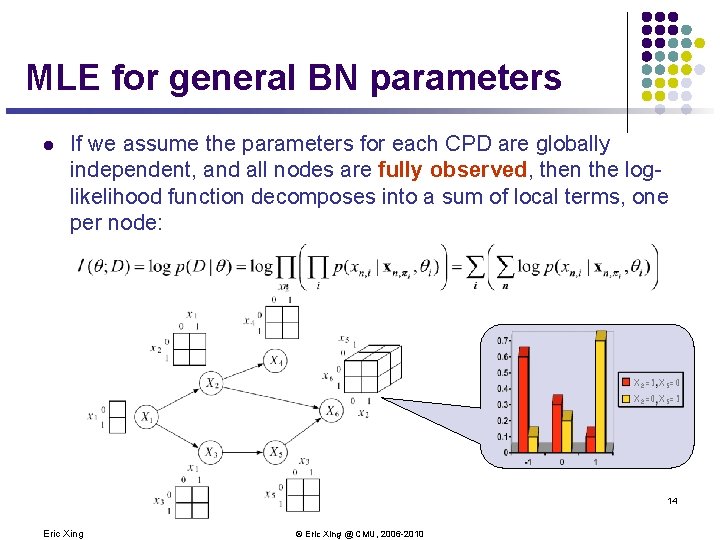
MLE for general BN parameters l If we assume the parameters for each CPD are globally independent, and all nodes are fully observed, then the loglikelihood function decomposes into a sum of local terms, one per node: X 2=1 X 5=0 X 2=0 X 5=1 14 Eric Xing © Eric Xing @ CMU, 2006 -2010

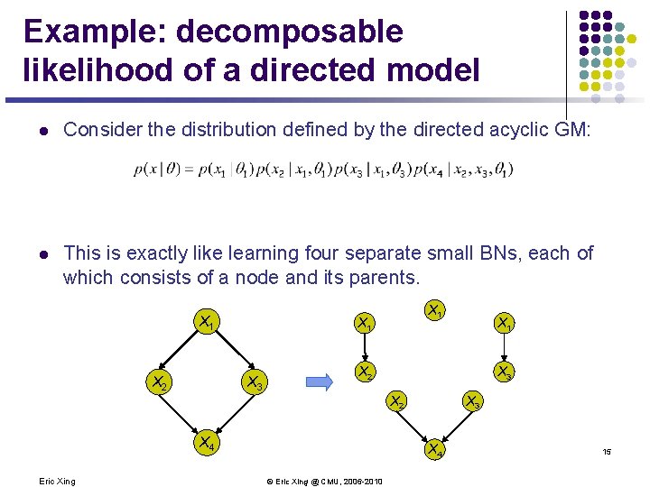
Example: decomposable likelihood of a directed model l Consider the distribution defined by the directed acyclic GM: l This is exactly like learning four separate small BNs, each of which consists of a node and its parents. X 1 X 2 X 3 X 2 X 4 Eric Xing X 1 X 3 X 4 © Eric Xing @ CMU, 2006 -2010 15

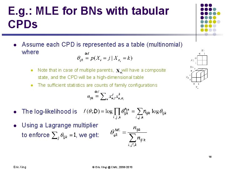
E. g. : MLE for BNs with tabular CPDs l Assume each CPD is represented as a table (multinomial) where l Note that in case of multiple parents, will have a composite state, and the CPD will be a high-dimensional table l The sufficient statistics are counts of family configurations l The log-likelihood is l Using a Lagrange multiplier to enforce , we get: 16 Eric Xing © Eric Xing @ CMU, 2006 -2010

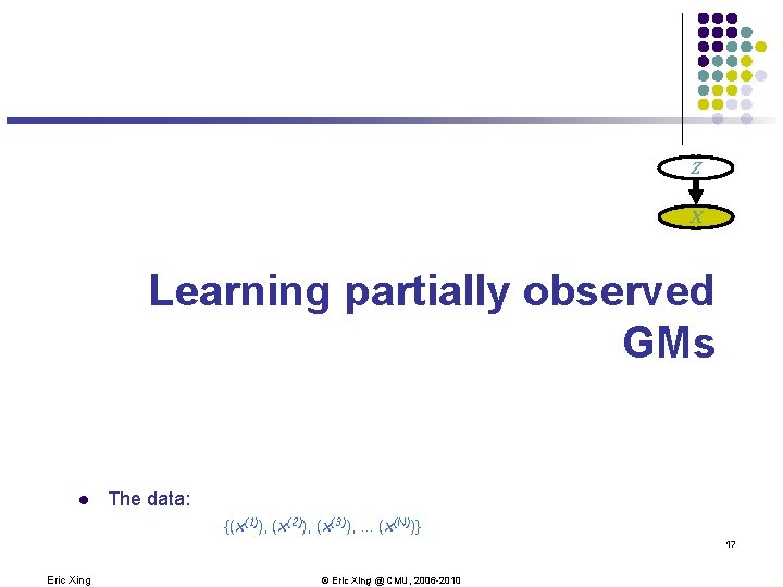
Z X Learning partially observed GMs l The data: {(x(1)), (x(2)), (x(3)), . . . (x(N))} 17 Eric Xing © Eric Xing @ CMU, 2006 -2010

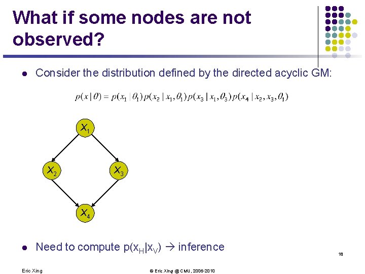
What if some nodes are not observed? l Consider the distribution defined by the directed acyclic GM: X 1 X 2 X 3 X 4 l Need to compute p(x. H|x. V) inference Eric Xing © Eric Xing @ CMU, 2006 -2010 18

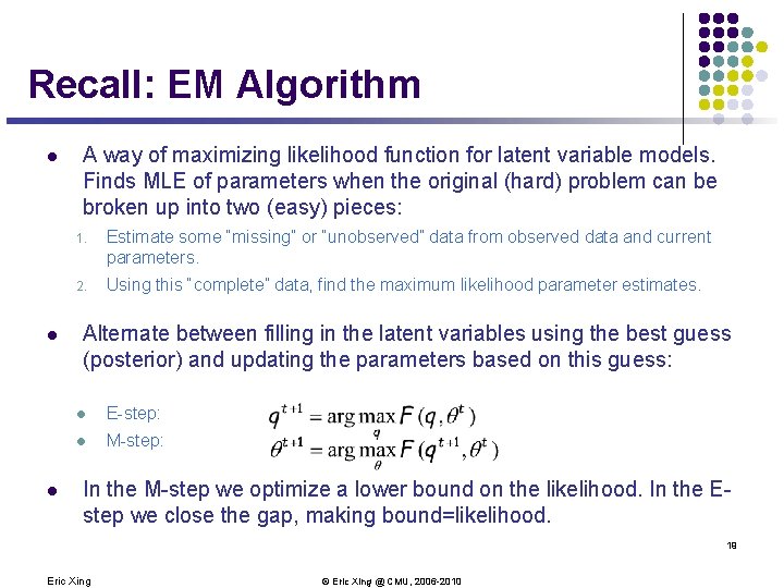
Recall: EM Algorithm l l l A way of maximizing likelihood function for latent variable models. Finds MLE of parameters when the original (hard) problem can be broken up into two (easy) pieces: 1. Estimate some “missing” or “unobserved” data from observed data and current parameters. 2. Using this “complete” data, find the maximum likelihood parameter estimates. Alternate between filling in the latent variables using the best guess (posterior) and updating the parameters based on this guess: l E-step: l M-step: In the M-step we optimize a lower bound on the likelihood. In the Estep we close the gap, making bound=likelihood. 19 Eric Xing © Eric Xing @ CMU, 2006 -2010

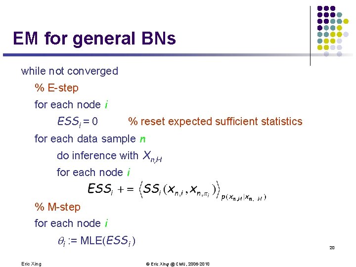
EM for general BNs while not converged % E-step for each node i ESSi = 0 % reset expected sufficient statistics for each data sample n do inference with Xn, H for each node i % M-step for each node i i : = MLE(ESSi ) Eric Xing 20 © Eric Xing @ CMU, 2006 -2010

Example: HMM l Supervised learning: estimation when the “right answer” is known l Examples: GIVEN: a genomic region x = x 1…x 1, 000 where we have good (experimental) annotations of the Cp. G islands GIVEN: the casino player allows us to observe him one evening, as he changes dice and produces 10, 000 rolls l Unsupervised learning: estimation when the “right answer” is unknown l Examples: GIVEN: l the porcupine genome; we don’t know how frequent are the Cp. G islands there, neither do we know their composition 10, 000 rolls of the casino player, but we don’t see when he changes dice QUESTION: Update the parameters of the model to maximize P(x| ) -- Maximal likelihood (ML) estimation 21 Eric Xing © Eric Xing @ CMU, 2006 -2010

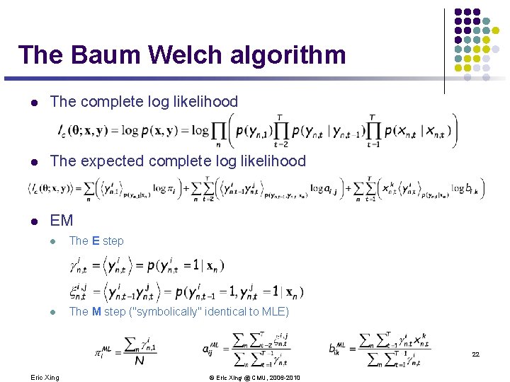
The Baum Welch algorithm l The complete log likelihood l The expected complete log likelihood l EM l The E step l The M step ("symbolically" identical to MLE) 22 Eric Xing © Eric Xing @ CMU, 2006 -2010

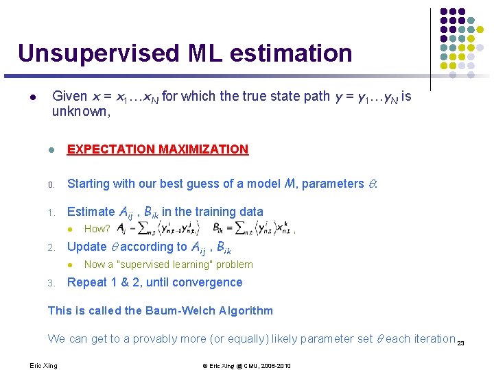
Unsupervised ML estimation l Given x = x 1…x. N for which the true state path y = y 1…y. N is unknown, l EXPECTATION MAXIMIZATION 0. Starting with our best guess of a model M, parameters : 1. Estimate Aij , Bik in the training data l 2. , , Update according to Aij , Bik l 3. How? Now a "supervised learning" problem Repeat 1 & 2, until convergence This is called the Baum-Welch Algorithm We can get to a provably more (or equally) likely parameter set each iteration 23 Eric Xing © Eric Xing @ CMU, 2006 -2010

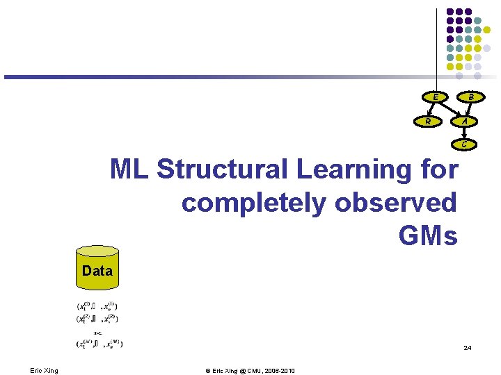
B E R A C ML Structural Learning for completely observed GMs Data 24 Eric Xing © Eric Xing @ CMU, 2006 -2010

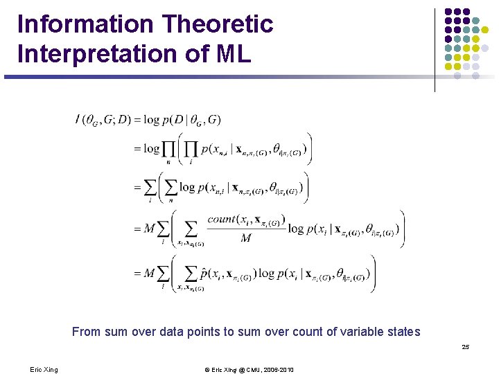
Information Theoretic Interpretation of ML From sum over data points to sum over count of variable states 25 Eric Xing © Eric Xing @ CMU, 2006 -2010

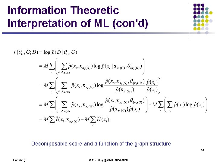
Information Theoretic Interpretation of ML (con'd) Decomposable score and a function of the graph structure 26 Eric Xing © Eric Xing @ CMU, 2006 -2010

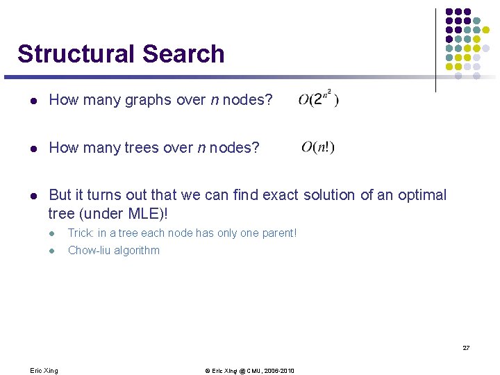
Structural Search l How many graphs over n nodes? l How many trees over n nodes? l But it turns out that we can find exact solution of an optimal tree (under MLE)! l Trick: in a tree each node has only one parent! l Chow-liu algorithm 27 Eric Xing © Eric Xing @ CMU, 2006 -2010

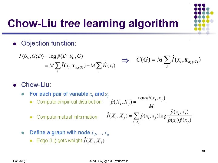
Chow-Liu tree learning algorithm l Objection function: Þ l Chow-Liu: l l For each pair of variable xi and xj l Compute empirical distribution: l Compute mutual information: Define a graph with node x 1, …, xn l Edge (I, j) gets weight 28 Eric Xing © Eric Xing @ CMU, 2006 -2010

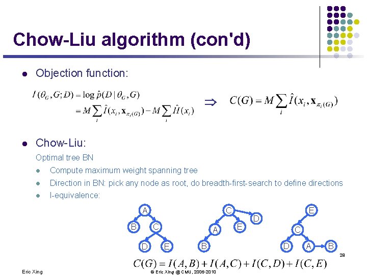
Chow-Liu algorithm (con'd) l Objection function: Þ l Chow-Liu: Optimal tree BN l Compute maximum weight spanning tree l Direction in BN: pick any node as root, do breadth-first-search to define directions l I-equivalence: C A B C D A E B E E D C D A B 29 Eric Xing © Eric Xing @ CMU, 2006 -2010

Structure Learning for general graphs l Theorem: l The problem of learning a BN structure with at most d parents is NP-hard for any (fixed) d≥ 2 l Most structure learning approaches use heuristics l Exploit score decomposition l Two heuristics that exploit decomposition in different ways l Greedy search through space of node-orders l Local search of graph structures 30 Eric Xing © Eric Xing @ CMU, 2006 -2010

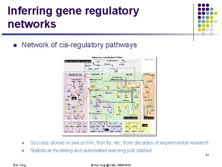
Inferring gene regulatory networks l Network of cis-regulatory pathways l Success stories in sea urchin, fruit fly, etc, from decades of experimental research l Statistical modeling and automated learning just started 31 Eric Xing © Eric Xing @ CMU, 2006 -2010

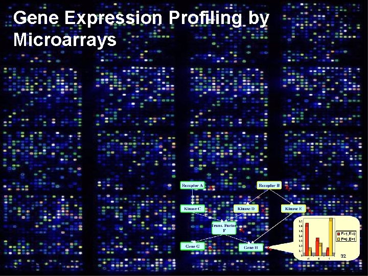
Gene Expression Profiling by Microarrays 32 Eric Xing © Eric Xing @ CMU, 2006 -2010

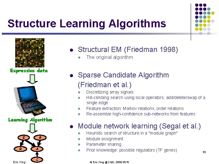
Structure Learning Algorithms l Structural EM (Friedman 1998) l Expression data l Sparse Candidate Algorithm (Friedman et al. ) l l Learning Algorithm l B E R Eric Xing A C The original algorithm Discretizing array signals Hill-climbing search using local operators: add/delete/swap of a single edge Feature extraction: Markov relations, order relations Re-assemble high-confidence sub-networks from features Module network learning (Segal et al. ) l l Heuristic search of structure in a "module graph" Module assignment Parameter sharing Prior knowledge: possible regulators (TF genes) © Eric Xing @ CMU, 2006 -2010 33

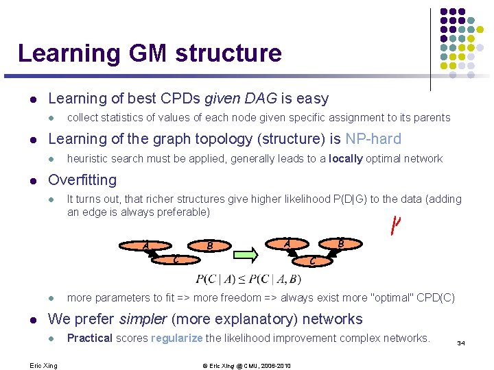
Learning GM structure l Learning of best CPDs given DAG is easy l l Learning of the graph topology (structure) is NP-hard l l collect statistics of values of each node given specific assignment to its parents heuristic search must be applied, generally leads to a locally optimal network Overfitting l It turns out, that richer structures give higher likelihood P(D|G) to the data (adding an edge is always preferable) A B A C l l B C more parameters to fit => more freedom => always exist more "optimal" CPD(C) We prefer simpler (more explanatory) networks l Eric Xing Practical scores regularize the likelihood improvement complex networks. © Eric Xing @ CMU, 2006 -2010 34

l Learning Graphical Model Structure via Neighborhood Selection 35 Eric Xing © Eric Xing @ CMU, 2006 -2010

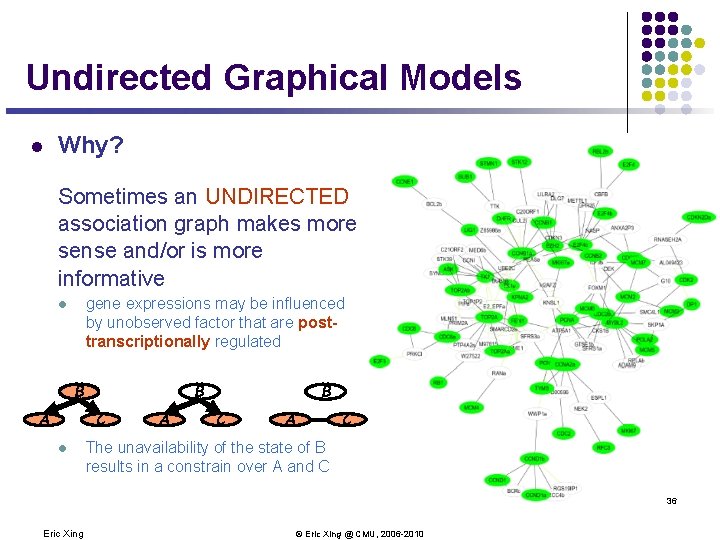
Undirected Graphical Models l Why? Sometimes an UNDIRECTED association graph makes more sense and/or is more informative gene expressions may be influenced by unobserved factor that are posttranscriptionally regulated l B B C A l A B C A C The unavailability of the state of B results in a constrain over A and C 36 Eric Xing © Eric Xing @ CMU, 2006 -2010

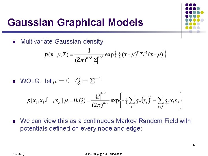
Gaussian Graphical Models l Multivariate Gaussian density: l WOLG: let l We can view this as a continuous Markov Random Field with potentials defined on every node and edge: 37 Eric Xing © Eric Xing @ CMU, 2006 -2010

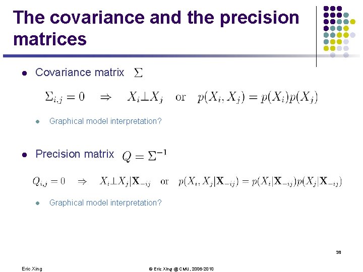
The covariance and the precision matrices l Covariance matrix l l Graphical model interpretation? Precision matrix l Graphical model interpretation? 38 Eric Xing © Eric Xing @ CMU, 2006 -2010

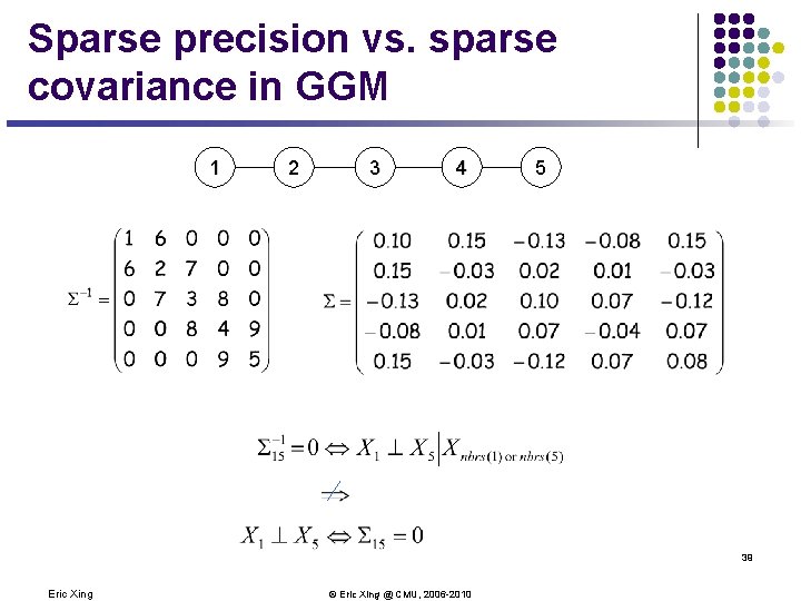
Sparse precision vs. sparse covariance in GGM 1 2 3 4 5 39 Eric Xing © Eric Xing @ CMU, 2006 -2010

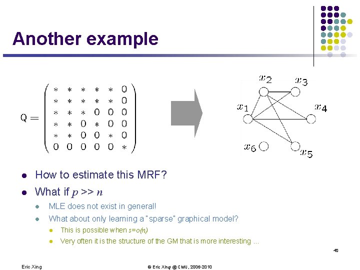
Another example l How to estimate this MRF? l What if p >> n l MLE does not exist in general! l What about only learning a “sparse” graphical model? l This is possible when s=o(n) l Very often it is the structure of the GM that is more interesting … 40 Eric Xing © Eric Xing @ CMU, 2006 -2010

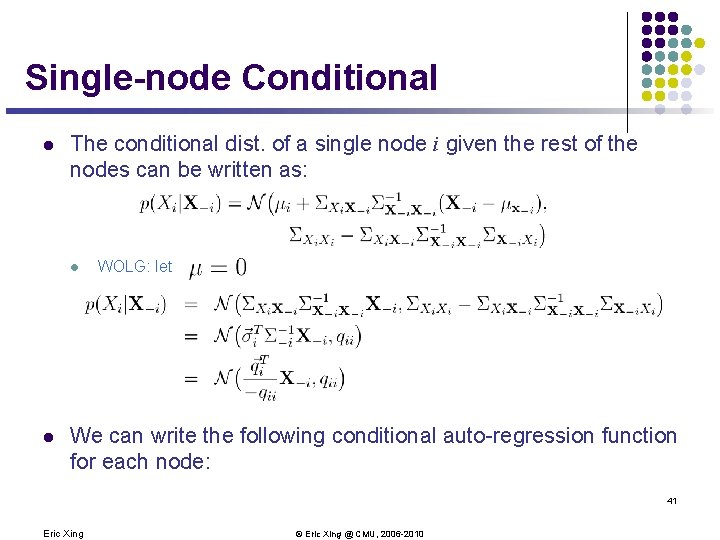
Single-node Conditional l The conditional dist. of a single node i given the rest of the nodes can be written as: l l WOLG: let We can write the following conditional auto-regression function for each node: 41 Eric Xing © Eric Xing @ CMU, 2006 -2010

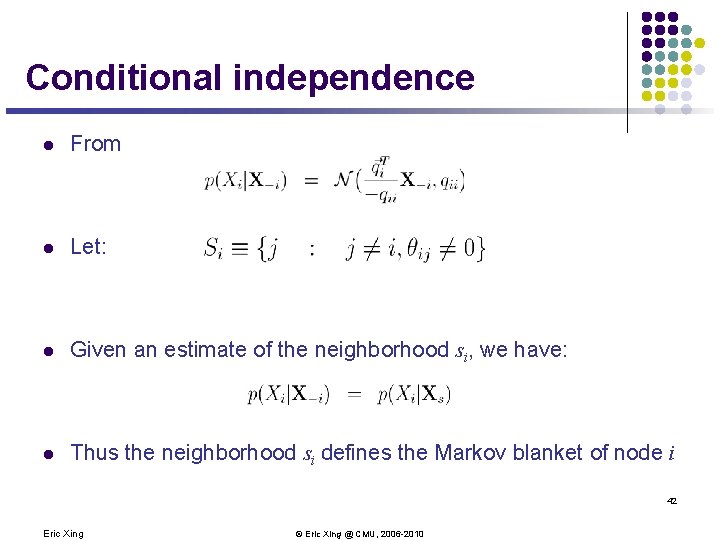
Conditional independence l From l Let: l Given an estimate of the neighborhood si, we have: l Thus the neighborhood si defines the Markov blanket of node i 42 Eric Xing © Eric Xing @ CMU, 2006 -2010

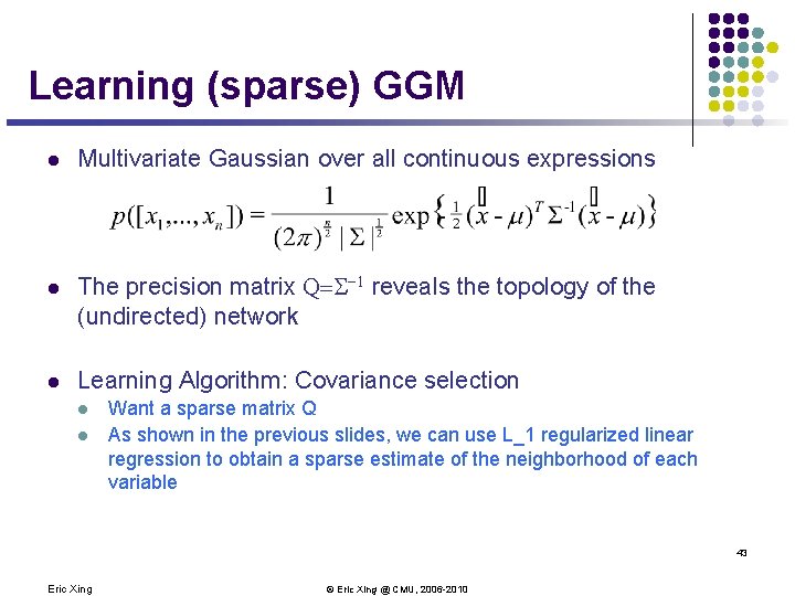
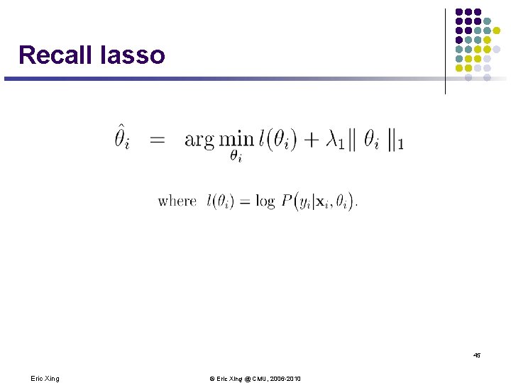
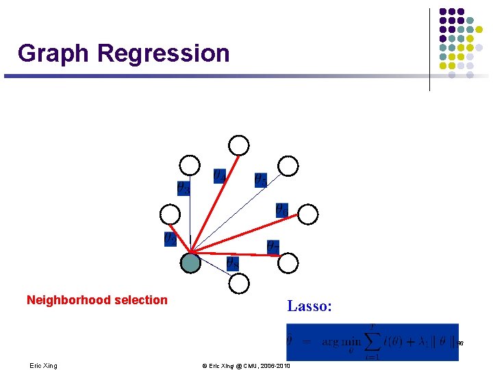
Learning (sparse) GGM l Multivariate Gaussian over all continuous expressions l The precision matrix Q=S-1 reveals the topology of the (undirected) network l Learning Algorithm: Covariance selection l l Want a sparse matrix Q As shown in the previous slides, we can use L_1 regularized linear regression to obtain a sparse estimate of the neighborhood of each variable 43 Eric Xing © Eric Xing @ CMU, 2006 -2010

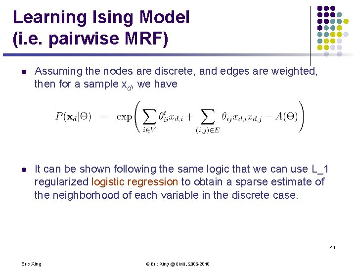
Learning Ising Model (i. e. pairwise MRF) l Assuming the nodes are discrete, and edges are weighted, then for a sample xd, we have l It can be shown following the same logic that we can use L_1 regularized logistic regression to obtain a sparse estimate of the neighborhood of each variable in the discrete case. 44 Eric Xing © Eric Xing @ CMU, 2006 -2010

Recall lasso 45 Eric Xing © Eric Xing @ CMU, 2006 -2010

Graph Regression Neighborhood selection Lasso: 46 Eric Xing © Eric Xing @ CMU, 2006 -2010

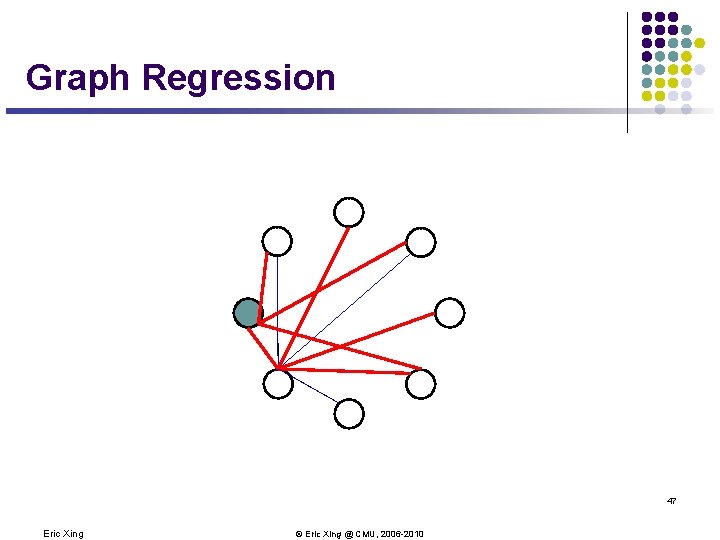
Graph Regression 47 Eric Xing © Eric Xing @ CMU, 2006 -2010

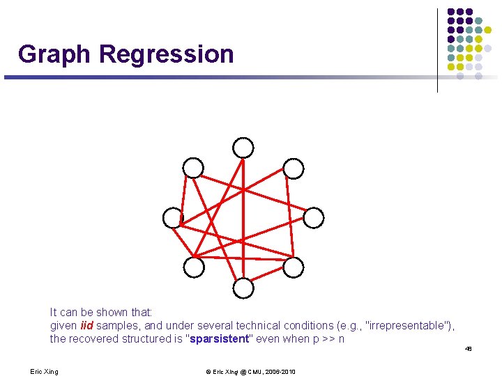
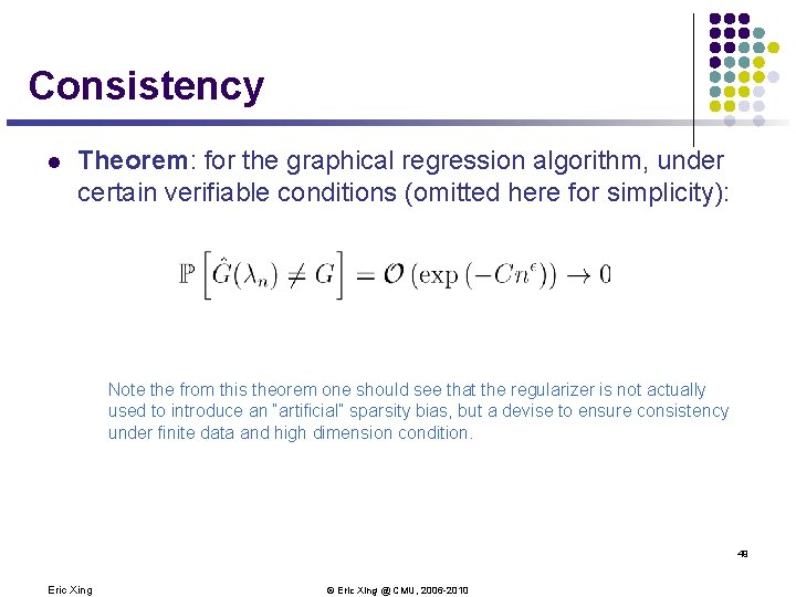
Graph Regression It can be shown that: given iid samples, and under several technical conditions (e. g. , "irrepresentable"), the recovered structured is "sparsistent" even when p >> n 48 Eric Xing © Eric Xing @ CMU, 2006 -2010

Consistency l Theorem: for the graphical regression algorithm, under certain verifiable conditions (omitted here for simplicity): Note the from this theorem one should see that the regularizer is not actually used to introduce an “artificial” sparsity bias, but a devise to ensure consistency under finite data and high dimension condition. 49 Eric Xing © Eric Xing @ CMU, 2006 -2010

Recent trends in GGM: l Covariance selection (classical method) l Dempster [1972]: l l l L 1 -regularization based method (hot !) Meinshausen and Bühlmann [Ann. Stat. 06]: l Sequentially pruning smallest elements in precision matrix l Drton and Perlman [2008]: l Improved statistical tests for pruning Banerjee [JMLR 08]: l l Block sub-gradient algorithm for finding precision matrix Friedman et al. [Biostatistics 08]: l l Serious limitations in practice: breaks down when covariance matrix is not invertible Used LASSO regression for neighborhood selection Efficient fixed-point equations based on a sub-gradient algorithm … l Structure learning is possible even when # variables ＞ # samples Eric Xing © Eric Xing @ CMU, 2006 -2010 50

Learning GM l Learning of best CPDs given DAG is easy l l Learning of the graph topology (structure) is NP-hard l l collect statistics of values of each node given specific assignment to its parents heuristic search must be applied, generally leads to a locally optimal network We prefer simpler (more explanatory) networks l Regularized graph regression 51 Eric Xing © Eric Xing @ CMU, 2006 -2010