Machine Learning for Signal Processing Principal Component Analysis


![Eigen faces eigenface 1 eigenface 2 [U, S] = eig(correlation) • Compute the eigen Eigen faces eigenface 1 eigenface 2 [U, S] = eig(correlation) • Compute the eigen](https://slidetodoc.com/presentation_image/79c53b54322e1f7a61844a9964a21364/image-38.jpg)
![Using SVD to compute Eigenbases [U, S, V] = SVD(X) • U will have Using SVD to compute Eigenbases [U, S, V] = SVD(X) • U will have](https://slidetodoc.com/presentation_image/79c53b54322e1f7a61844a9964a21364/image-60.jpg)


- Slides: 80

Machine Learning for Signal Processing Principal Component Analysis Class 7. 12 Feb 2015 Instructor: Bhiksha Raj 9/25/2020 11 -755/18 -797 1

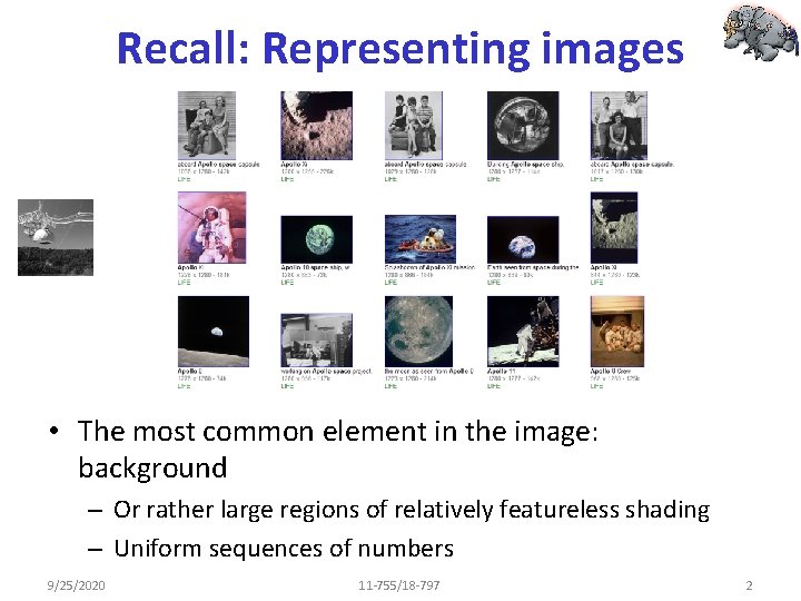
Recall: Representing images • The most common element in the image: background – Or rather large regions of relatively featureless shading – Uniform sequences of numbers 9/25/2020 11 -755/18 -797 2

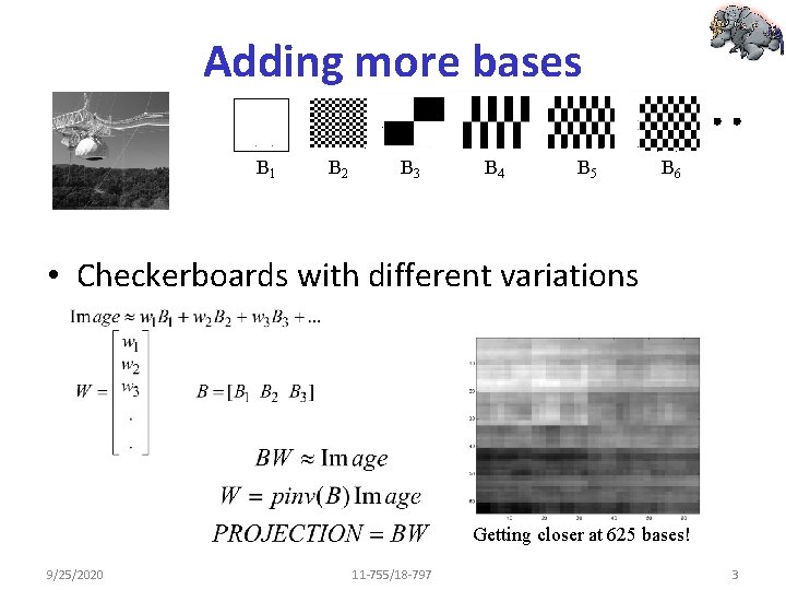
Adding more bases B 1 B 2 B 3 B 4 B 5 B 6 • Checkerboards with different variations Getting closer at 625 bases! 9/25/2020 11 -755/18 -797 3

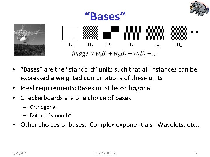
“Bases” B 1 B 2 B 3 B 4 B 5 B 6 • “Bases” are the “standard” units such that all instances can be expressed a weighted combinations of these units • Ideal requirements: Bases must be orthogonal • Checkerboards are one choice of bases – Orthogonal – But not “smooth” • Other choices of bases: Complex exponentials, Wavelets, etc. . 9/25/2020 11 -755/18 -797 4

Data specific bases? • Issue: All the bases we have considered so far are data agnostic – Checkerboards, Complex exponentials, Wavelets. . – We use the same bases regardless of the data we analyze • Image of face vs. Image of a forest • Segment of speech vs. Seismic rumble • How about data specific bases – Bases that consider the underlying data • E. g. is there something better than checkerboards to describe faces • Something better than complex exponentials to describe music? 9/25/2020 11 -755/18 -797 5

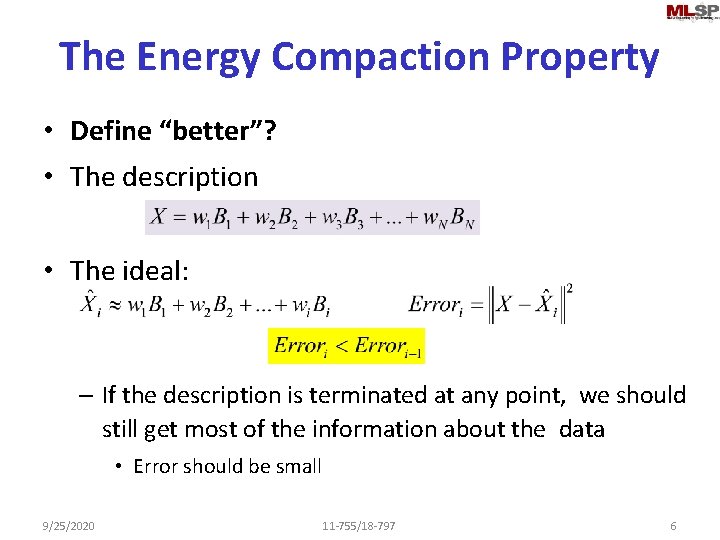
The Energy Compaction Property • Define “better”? • The description • The ideal: – If the description is terminated at any point, we should still get most of the information about the data • Error should be small 9/25/2020 11 -755/18 -797 6

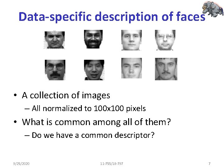
Data-specific description of faces • A collection of images – All normalized to 100 x 100 pixels • What is common among all of them? – Do we have a common descriptor? 9/25/2020 11 -755/18 -797 7

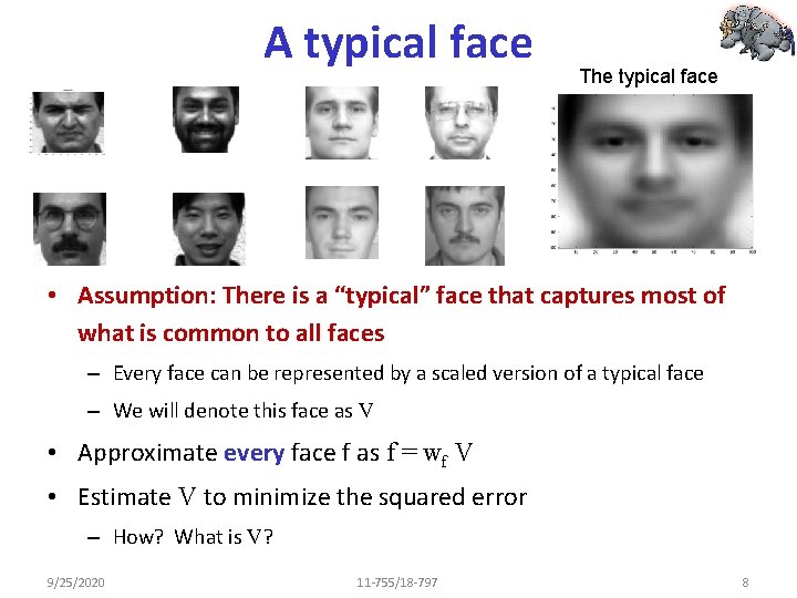
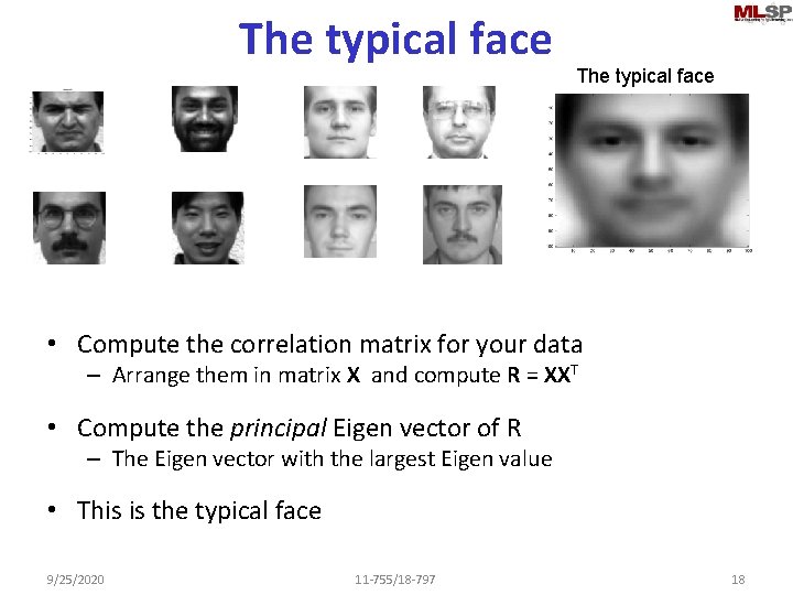
A typical face The typical face • Assumption: There is a “typical” face that captures most of what is common to all faces – Every face can be represented by a scaled version of a typical face – We will denote this face as V • Approximate every face f as f = wf V • Estimate V to minimize the squared error – How? What is V? 9/25/2020 11 -755/18 -797 8

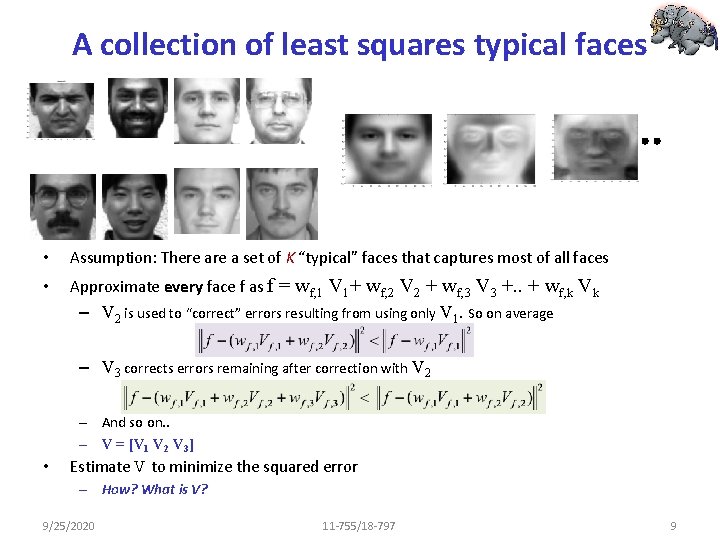
A collection of least squares typical faces • Assumption: There a set of K “typical” faces that captures most of all faces • Approximate every face f as f = wf, 1 V 1+ wf, 2 V 2 + wf, 3 V 3 +. . + wf, k Vk – V 2 is used to “correct” errors resulting from using only V 1. So on average – V 3 corrects errors remaining after correction with V 2 – And so on. . – V = [V 1 V 2 V 3] • Estimate V to minimize the squared error – How? What is V? 9/25/2020 11 -755/18 -797 9

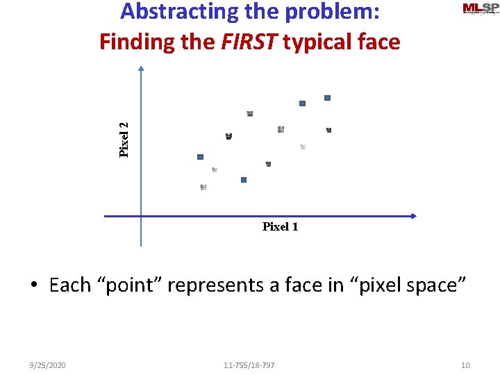
Pixel 2 Abstracting the problem: Finding the FIRST typical face Pixel 1 • Each “point” represents a face in “pixel space” 9/25/2020 11 -755/18 -797 10

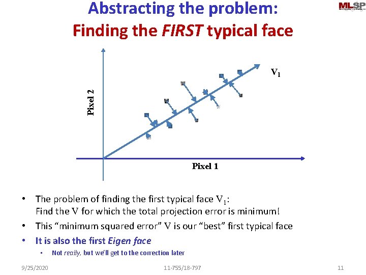
Abstracting the problem: Finding the FIRST typical face Pixel 2 V 1 Pixel 1 • The problem of finding the first typical face V 1: Find the V for which the total projection error is minimum! • This “minimum squared error” V is our “best” first typical face • It is also the first Eigen face • 9/25/2020 Not really, but we’ll get to the correction later 11 -755/18 -797 11

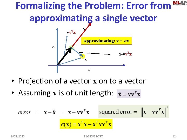
Formalizing the Problem: Error from approximating a single vector vv. Tx v y Approximating: x = wv x-vv. Tx x x • Projection of a vector x on to a vector • Assuming v is of unit length: 9/25/2020 11 -755/18 -797 12

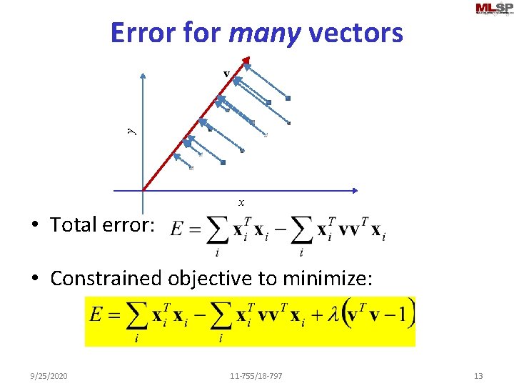
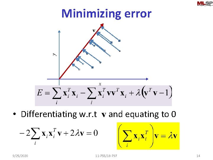
Error for many vectors y v x • Total error: • Constrained objective to minimize: 9/25/2020 11 -755/18 -797 13

Minimizing error y v x • Differentiating w. r. t v and equating to 0 9/25/2020 11 -755/18 -797 14

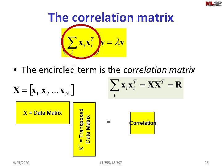
The correlation matrix X = Data Matrix 9/25/2020 XT = Transposed Data Matrix • The encircled term is the correlation matrix = 11 -755/18 -797 Correlation 15

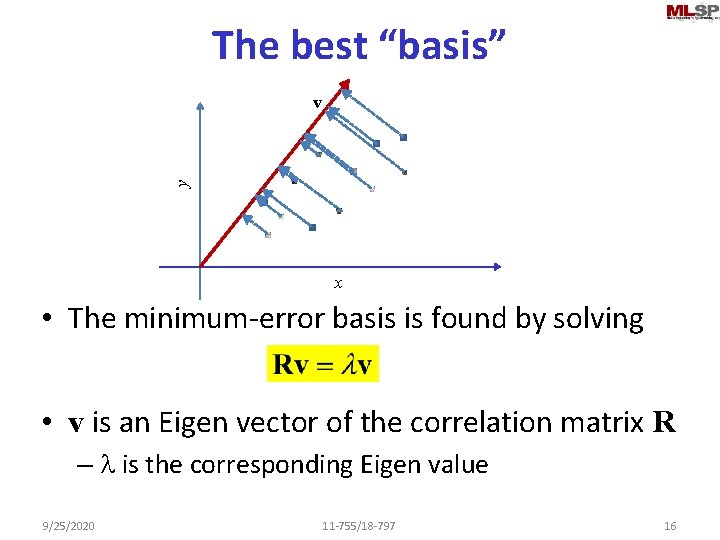
The best “basis” y v x • The minimum-error basis is found by solving • v is an Eigen vector of the correlation matrix R – l is the corresponding Eigen value 9/25/2020 11 -755/18 -797 16

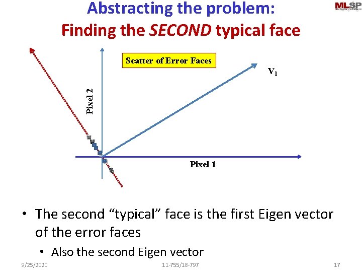
Abstracting the problem: Finding the SECOND typical face Scatter of Error Faces Pixel 2 V 1 Pixel 1 • The second “typical” face is the first Eigen vector of the error faces • Also the second Eigen vector 9/25/2020 11 -755/18 -797 17

The typical face • Compute the correlation matrix for your data – Arrange them in matrix X and compute R = XXT • Compute the principal Eigen vector of R – The Eigen vector with the largest Eigen value • This is the typical face 9/25/2020 11 -755/18 -797 18

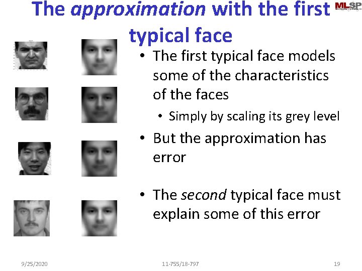
The approximation with the first typical face • The first typical face models some of the characteristics of the faces • Simply by scaling its grey level • But the approximation has error • The second typical face must explain some of this error 9/25/2020 11 -755/18 -797 19

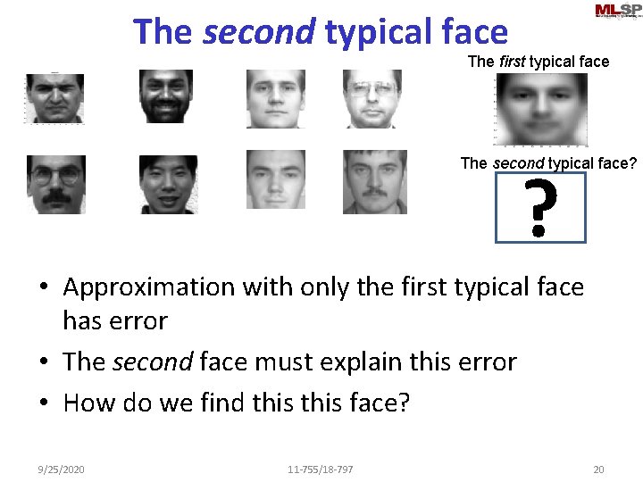
The second typical face The first typical face The second typical face? ? • Approximation with only the first typical face has error • The second face must explain this error • How do we find this face? 9/25/2020 11 -755/18 -797 20

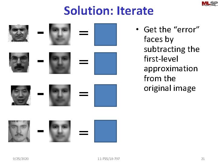
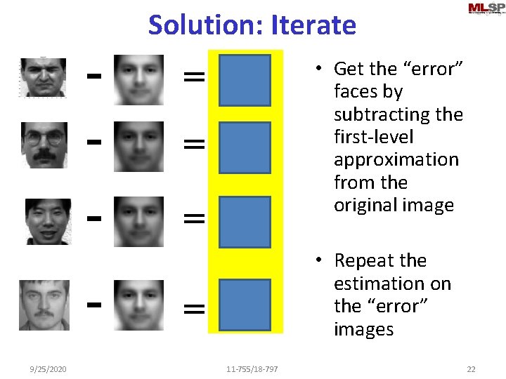
Solution: Iterate - = 9/25/2020 • Get the “error” faces by subtracting the first-level approximation from the original image = • Repeat the estimation on the “error” images = 11 -755/18 -797 21

Solution: Iterate - = 9/25/2020 • Get the “error” faces by subtracting the first-level approximation from the original image = • Repeat the estimation on the “error” images = 11 -755/18 -797 22

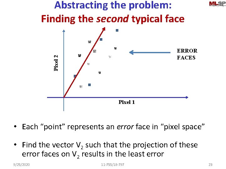
Abstracting the problem: Finding the second typical face Pixel 2 ERROR FACES Pixel 1 • Each “point” represents an error face in “pixel space” • Find the vector V 2 such that the projection of these error faces on V 2 results in the least error 9/25/2020 11 -755/18 -797 23

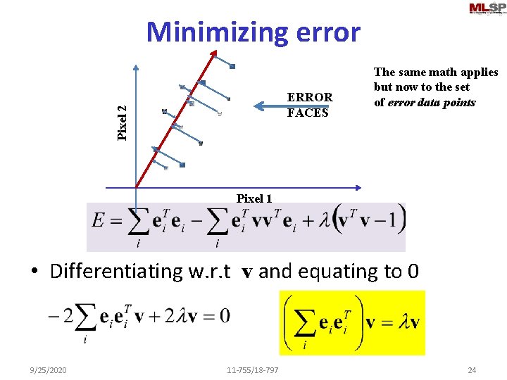
Minimizing error Pixel 2 ERROR FACES The same math applies but now to the set of error data points Pixel 1 • Differentiating w. r. t v and equating to 0 9/25/2020 11 -755/18 -797 24

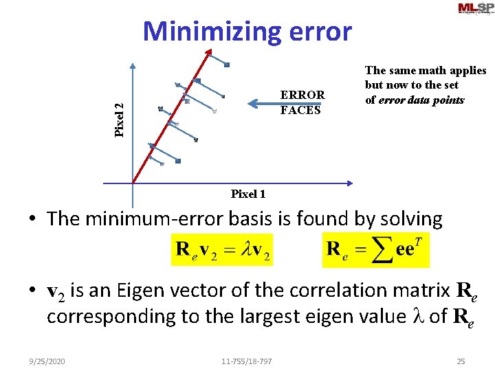
Minimizing error Pixel 2 ERROR FACES The same math applies but now to the set of error data points Pixel 1 • The minimum-error basis is found by solving • v 2 is an Eigen vector of the correlation matrix Re corresponding to the largest eigen value l of Re 9/25/2020 11 -755/18 -797 25

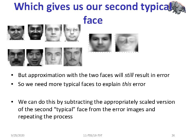
Which gives us our second typical face • But approximation with the two faces will still result in error • So we need more typical faces to explain this error • We can do this by subtracting the appropriately scaled version of the second “typical” face from the error images and repeating the process 9/25/2020 11 -755/18 -797 26

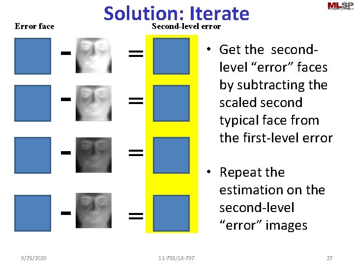
Error face 9/25/2020 - Solution: Iterate Second-level error = • Get the secondlevel “error” faces by subtracting the scaled second typical face from the first-level error = - = • Repeat the estimation on the second-level “error” images 11 -755/18 -797 27

An interesting property • Each “typical face” will be orthogonal to all other typical faces – Because each of them is learned to explain what the rest could not – None of these faces can explain one another! 9/25/2020 11 -755/18 -797 28

To add more faces • We can continue the process, refining the error each time – An instance of a procedure is called “Gram. Schmidt” orthogonalization • OR… we can do it all at once 9/25/2020 11 -755/18 -797 29

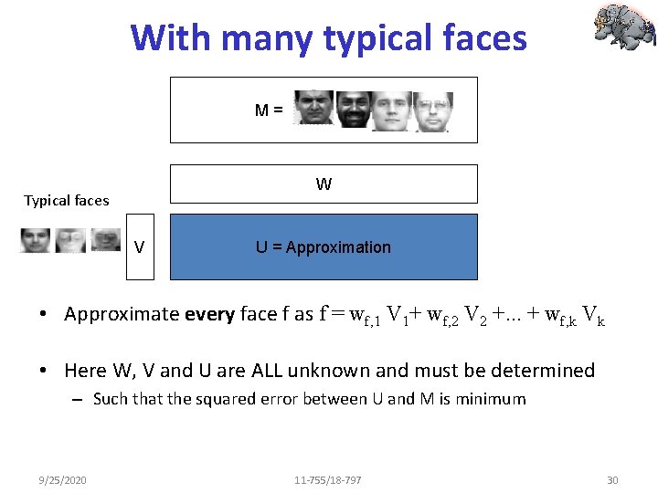
With many typical faces M= W Typical faces V U = Approximation • Approximate every face f as f = wf, 1 V 1+ wf, 2 V 2 +. . . + wf, k Vk • Here W, V and U are ALL unknown and must be determined – Such that the squared error between U and M is minimum 9/25/2020 11 -755/18 -797 30

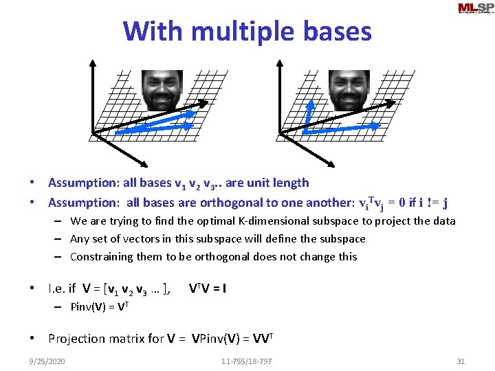
With multiple bases • Assumption: all bases v 1 v 2 v 3. . are unit length • Assumption: all bases are orthogonal to one another: vi. Tvj = 0 if i != j – We are trying to find the optimal K-dimensional subspace to project the data – Any set of vectors in this subspace will define the subspace – Constraining them to be orthogonal does not change this • I. e. if V = [v 1 v 2 v 3 … ], VTV = I – Pinv(V) = VT • Projection matrix for V = VPinv(V) = VVT 9/25/2020 11 -755/18 -797 31

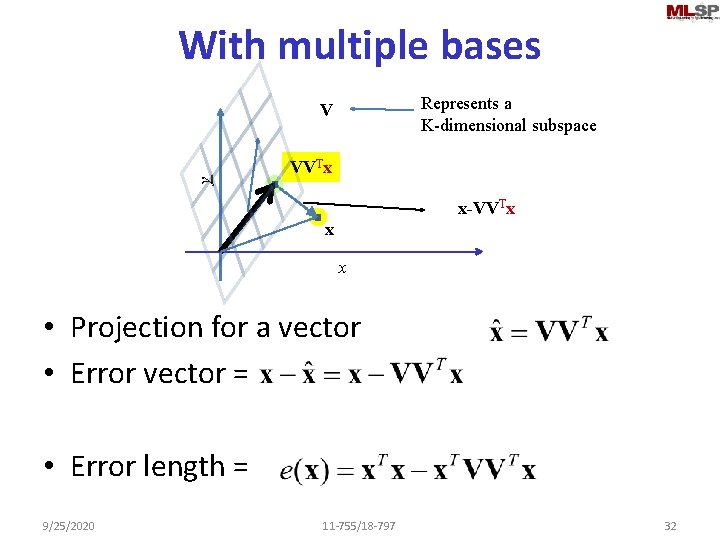
With multiple bases Represents a K-dimensional subspace y V VVTx x-VVTx x x • Projection for a vector • Error vector = • Error length = 9/25/2020 11 -755/18 -797 32

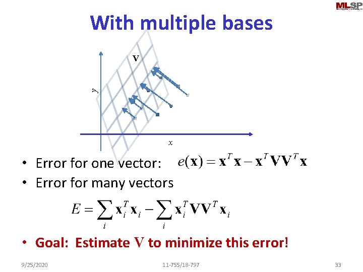
With multiple bases y V x • Error for one vector: • Error for many vectors • Goal: Estimate V to minimize this error! 9/25/2020 11 -755/18 -797 33

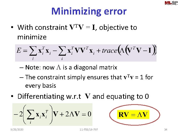
Minimizing error • With constraint VTV = I, objective to minimize – Note: now L is a diagonal matrix – The constraint simply ensures that v. Tv = 1 for every basis • Differentiating w. r. t V and equating to 0 9/25/2020 11 -755/18 -797 34

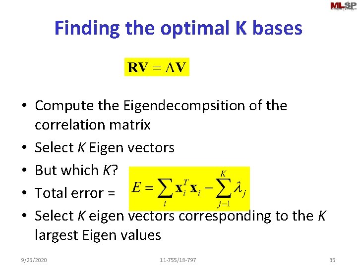
Finding the optimal K bases • Compute the Eigendecompsition of the correlation matrix • Select K Eigen vectors • But which K? • Total error = • Select K eigen vectors corresponding to the K largest Eigen values 9/25/2020 11 -755/18 -797 35

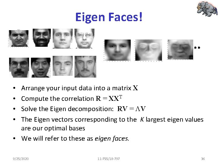
Eigen Faces! Arrange your input data into a matrix X Compute the correlation R = XXT Solve the Eigen decomposition: RV = LV The Eigen vectors corresponding to the K largest eigen values are our optimal bases • We will refer to these as eigen faces. • • 9/25/2020 11 -755/18 -797 36

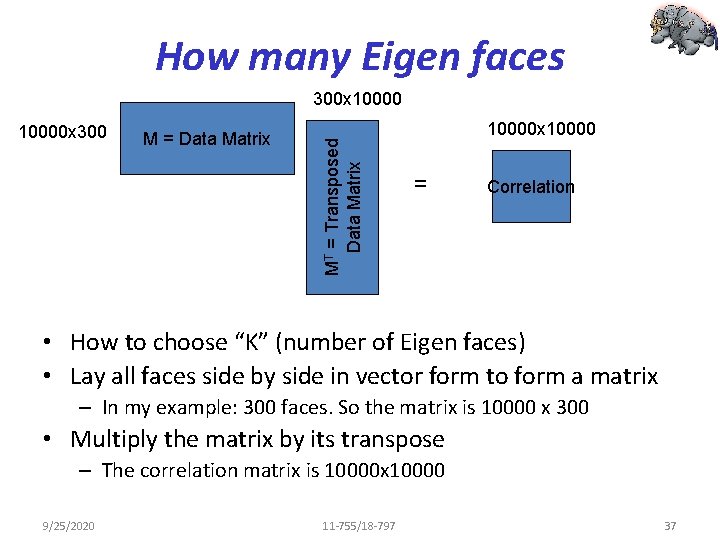
How many Eigen faces 10000 x 300 M = Data Matrix MT = Transposed Data Matrix 300 x 10000 x 10000 = Correlation • How to choose “K” (number of Eigen faces) • Lay all faces side by side in vector form to form a matrix – In my example: 300 faces. So the matrix is 10000 x 300 • Multiply the matrix by its transpose – The correlation matrix is 10000 x 10000 9/25/2020 11 -755/18 -797 37
![Eigen faces eigenface 1 eigenface 2 U S eigcorrelation Compute the eigen Eigen faces eigenface 1 eigenface 2 [U, S] = eig(correlation) • Compute the eigen](https://slidetodoc.com/presentation_image/79c53b54322e1f7a61844a9964a21364/image-38.jpg)
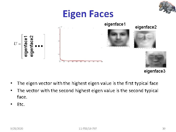
Eigen faces eigenface 1 eigenface 2 [U, S] = eig(correlation) • Compute the eigen vectors – Only 300 of the 10000 eigen values are non-zero • Why? • Retain eigen vectors with high eigen values (>0) – Could use a higher threshold 9/25/2020 11 -755/18 -797 38

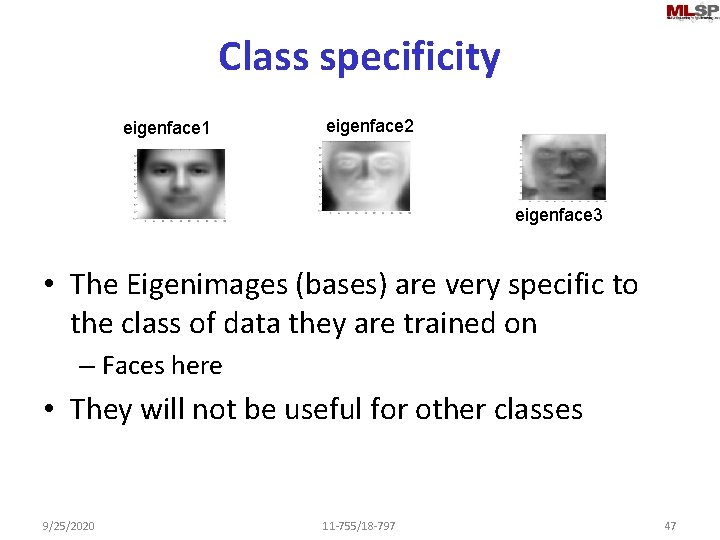
Eigen Faces eigenface 2 eigenface 1 eigenface 3 • The eigen vector with the highest eigen value is the first typical face • The vector with the second highest eigen value is the second typical face. • Etc. 9/25/2020 11 -755/18 -797 39

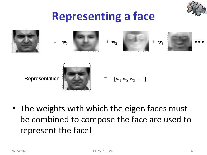
Representing a face = Representation w 1 + w 2 = + w 3 [w 1 w 2 w 3 …. ]T • The weights with which the eigen faces must be combined to compose the face are used to represent the face! 9/25/2020 11 -755/18 -797 40

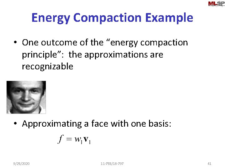
Energy Compaction Example • One outcome of the “energy compaction principle”: the approximations are recognizable • Approximating a face with one basis: 9/25/2020 11 -755/18 -797 41

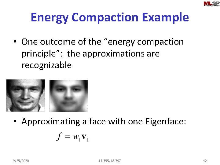
Energy Compaction Example • One outcome of the “energy compaction principle”: the approximations are recognizable • Approximating a face with one Eigenface: 9/25/2020 11 -755/18 -797 42

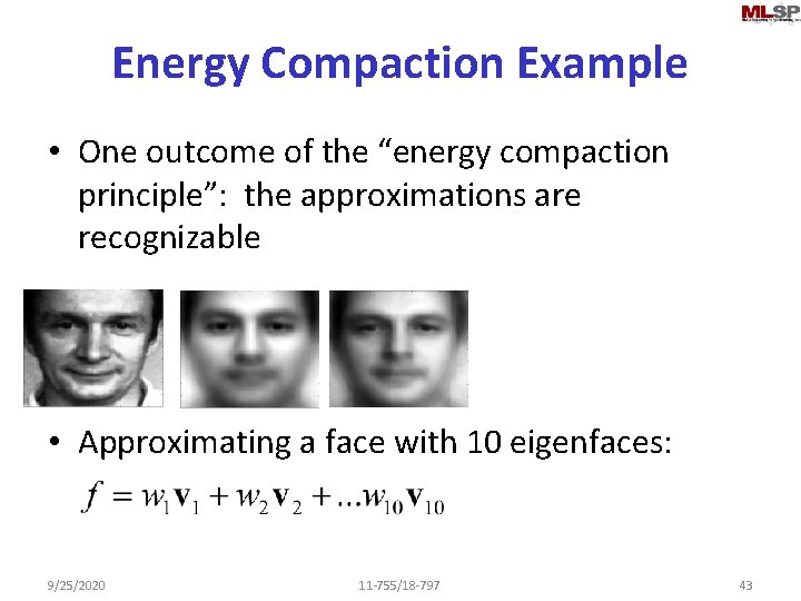
Energy Compaction Example • One outcome of the “energy compaction principle”: the approximations are recognizable • Approximating a face with 10 eigenfaces: 9/25/2020 11 -755/18 -797 43

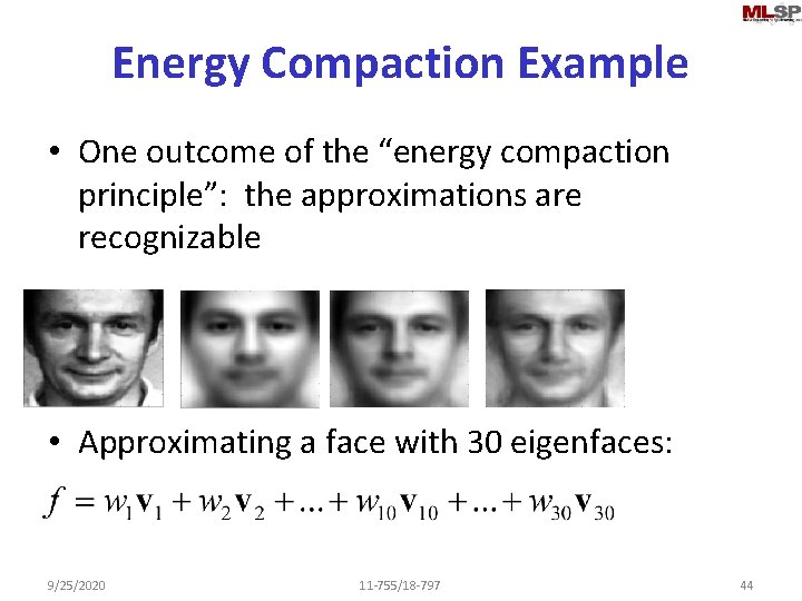
Energy Compaction Example • One outcome of the “energy compaction principle”: the approximations are recognizable • Approximating a face with 30 eigenfaces: 9/25/2020 11 -755/18 -797 44

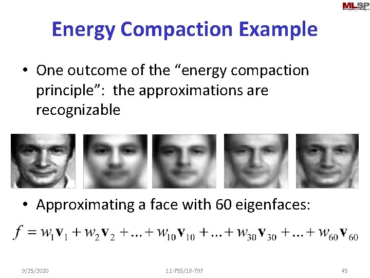
Energy Compaction Example • One outcome of the “energy compaction principle”: the approximations are recognizable • Approximating a face with 60 eigenfaces: 9/25/2020 11 -755/18 -797 45

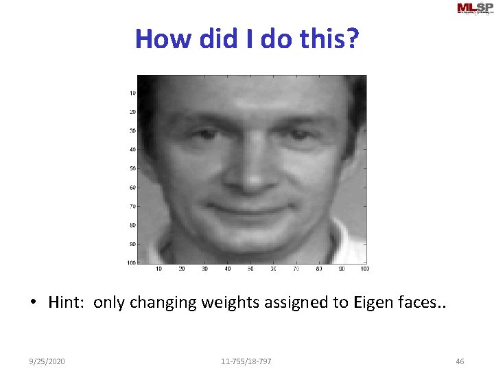
How did I do this? • Hint: only changing weights assigned to Eigen faces. . 9/25/2020 11 -755/18 -797 46

Class specificity eigenface 1 eigenface 2 eigenface 3 • The Eigenimages (bases) are very specific to the class of data they are trained on – Faces here • They will not be useful for other classes 9/25/2020 11 -755/18 -797 47

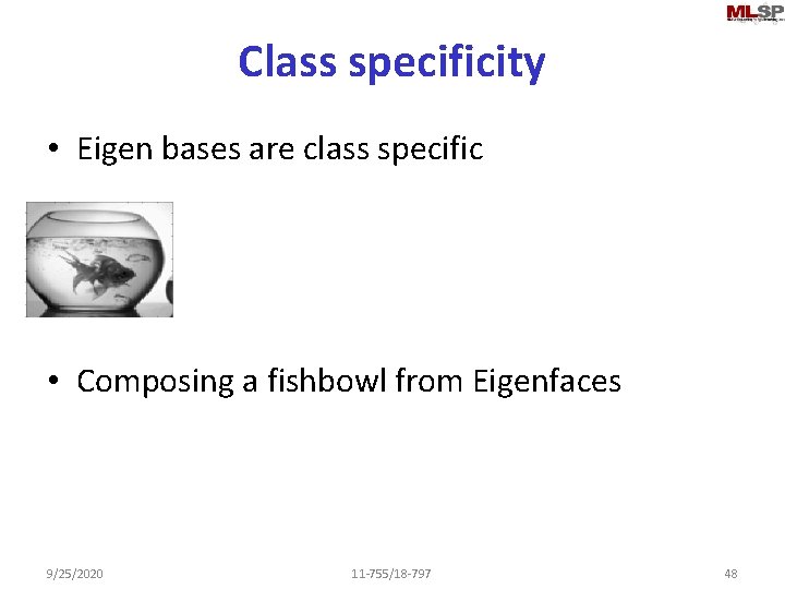
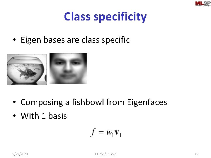
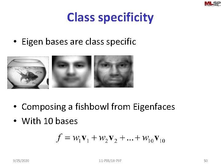
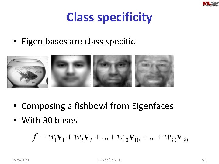
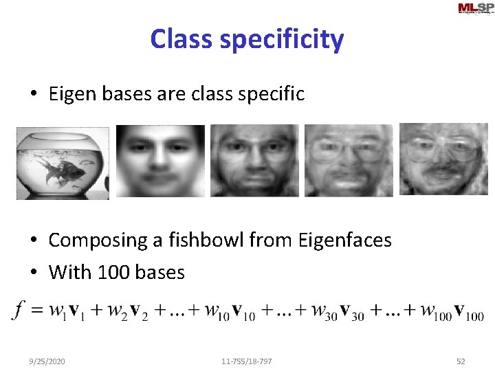
Class specificity • Eigen bases are class specific • Composing a fishbowl from Eigenfaces 9/25/2020 11 -755/18 -797 48

Class specificity • Eigen bases are class specific • Composing a fishbowl from Eigenfaces • With 1 basis 9/25/2020 11 -755/18 -797 49

Class specificity • Eigen bases are class specific • Composing a fishbowl from Eigenfaces • With 10 bases 9/25/2020 11 -755/18 -797 50

Class specificity • Eigen bases are class specific • Composing a fishbowl from Eigenfaces • With 30 bases 9/25/2020 11 -755/18 -797 51

Class specificity • Eigen bases are class specific • Composing a fishbowl from Eigenfaces • With 100 bases 9/25/2020 11 -755/18 -797 52

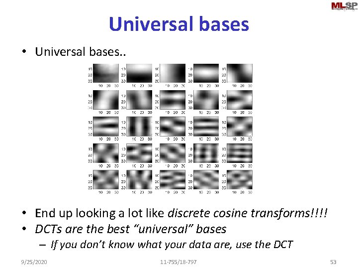
Universal bases • Universal bases. . • End up looking a lot like discrete cosine transforms!!!! • DCTs are the best “universal” bases – If you don’t know what your data are, use the DCT 9/25/2020 11 -755/18 -797 53

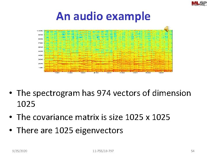
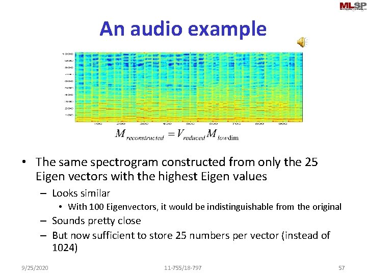
An audio example • The spectrogram has 974 vectors of dimension 1025 • The covariance matrix is size 1025 x 1025 • There are 1025 eigenvectors 9/25/2020 11 -755/18 -797 54

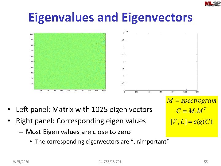
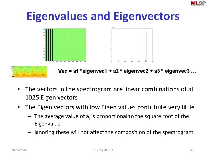
Eigenvalues and Eigenvectors • Left panel: Matrix with 1025 eigen vectors • Right panel: Corresponding eigen values – Most Eigen values are close to zero • The corresponding eigenvectors are “unimportant” 9/25/2020 11 -755/18 -797 55

Eigenvalues and Eigenvectors Vec = a 1 *eigenvec 1 + a 2 * eigenvec 2 + a 3 * eigenvec 3 … • The vectors in the spectrogram are linear combinations of all 1025 Eigen vectors • The Eigen vectors with low Eigen values contribute very little – The average value of ai is proportional to the square root of the Eigenvalue – Ignoring these will not affect the composition of the spectrogram 9/25/2020 11 -755/18 -797 56

An audio example • The same spectrogram constructed from only the 25 Eigen vectors with the highest Eigen values – Looks similar • With 100 Eigenvectors, it would be indistinguishable from the original – Sounds pretty close – But now sufficient to store 25 numbers per vector (instead of 1024) 9/25/2020 11 -755/18 -797 57

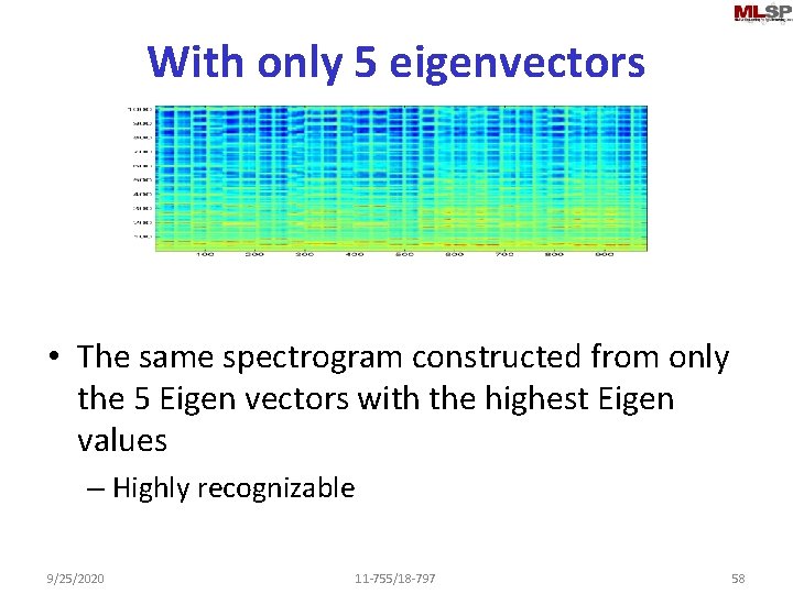
With only 5 eigenvectors • The same spectrogram constructed from only the 5 Eigen vectors with the highest Eigen values – Highly recognizable 9/25/2020 11 -755/18 -797 58

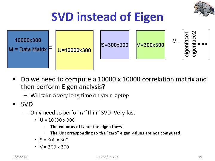
10000 x 300 M = Data Matrix = U=10000 x 300 S=300 x 300 V=300 x 300 eigenface 1 eigenface 2 SVD instead of Eigen • Do we need to compute a 10000 x 10000 correlation matrix and then perform Eigen analysis? – Will take a very long time on your laptop • SVD – Only need to perform “Thin” SVD. Very fast • U = 10000 x 300 – The columns of U are the eigen faces! – The Us corresponding to the “zero” eigen values are not computed • S = 300 x 300 • V = 300 x 300 9/25/2020 11 -755/18 -797 59
![Using SVD to compute Eigenbases U S V SVDX U will have Using SVD to compute Eigenbases [U, S, V] = SVD(X) • U will have](https://slidetodoc.com/presentation_image/79c53b54322e1f7a61844a9964a21364/image-60.jpg)
Using SVD to compute Eigenbases [U, S, V] = SVD(X) • U will have the Eigenvectors • Thin SVD for 100 bases: [U, S, V] = svds(X, 100) • Much more efficient 9/25/2020 11 -755/18 -797 60

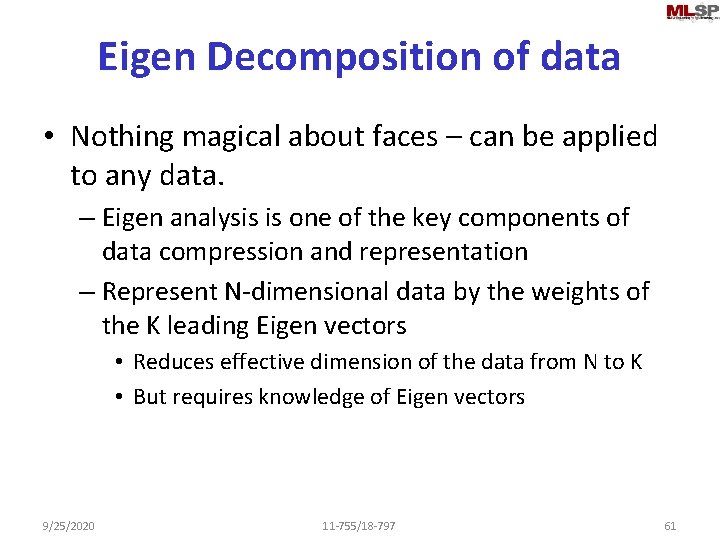
Eigen Decomposition of data • Nothing magical about faces – can be applied to any data. – Eigen analysis is one of the key components of data compression and representation – Represent N-dimensional data by the weights of the K leading Eigen vectors • Reduces effective dimension of the data from N to K • But requires knowledge of Eigen vectors 9/25/2020 11 -755/18 -797 61

Eigen decomposition of what? • Eigen decomposition of the correlation matrix • Is there an alternate way? 9/25/2020 11 -755/18 -797 62

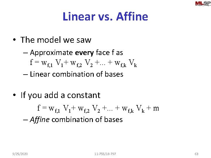
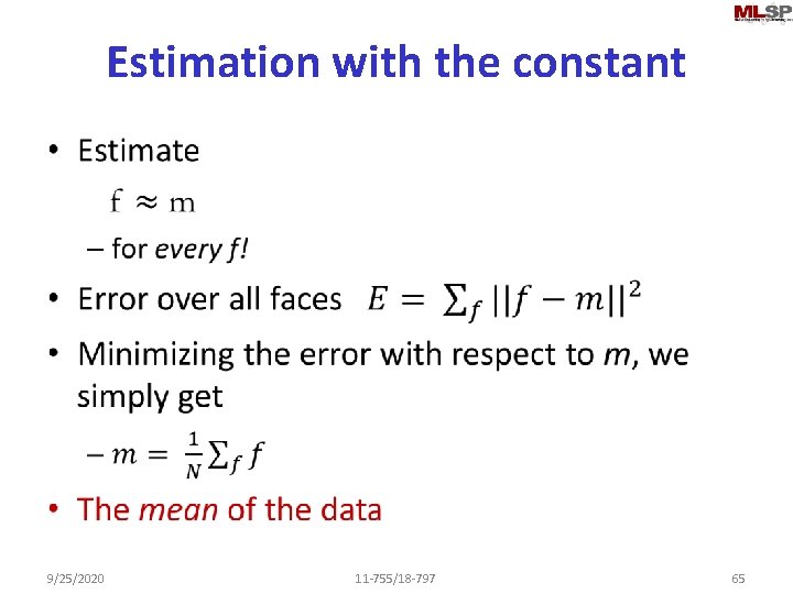
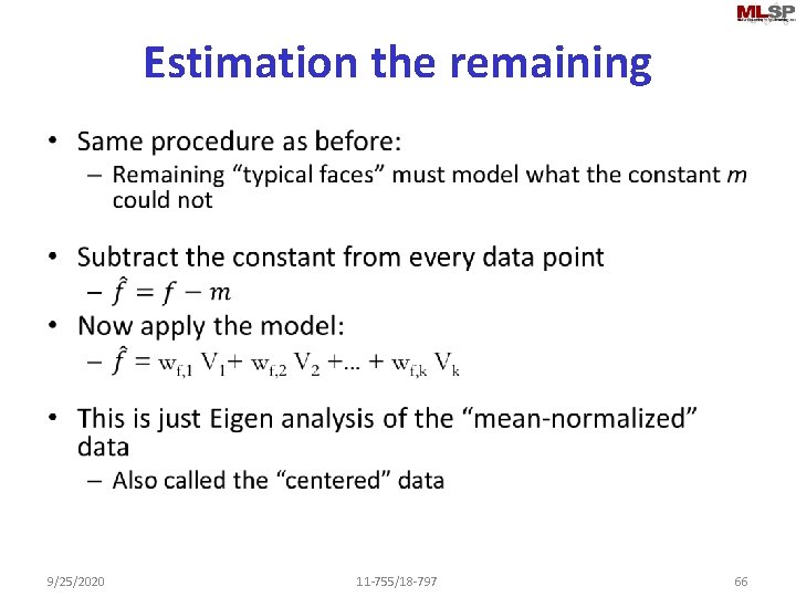
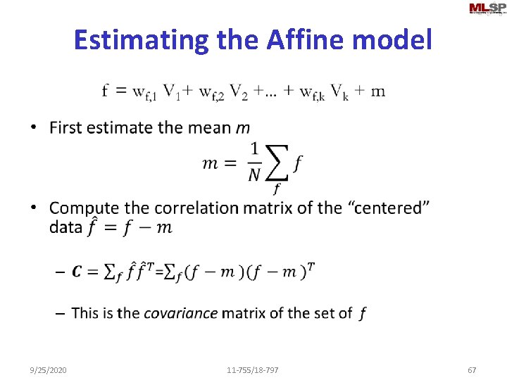
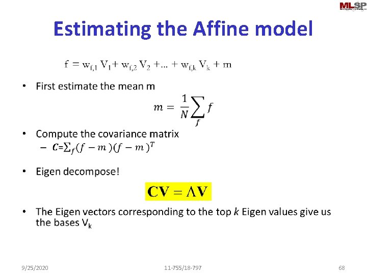
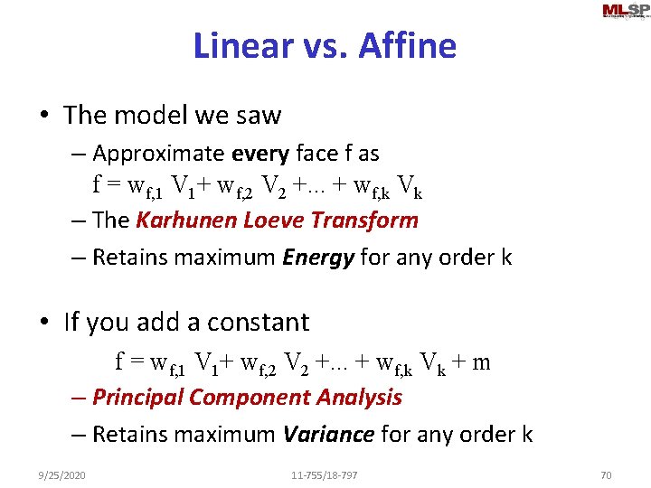
Linear vs. Affine • The model we saw – Approximate every face f as f = wf, 1 V 1+ wf, 2 V 2 +. . . + wf, k Vk – Linear combination of bases • If you add a constant f = wf, 1 V 1+ wf, 2 V 2 +. . . + wf, k Vk + m – Affine combination of bases 9/25/2020 11 -755/18 -797 63

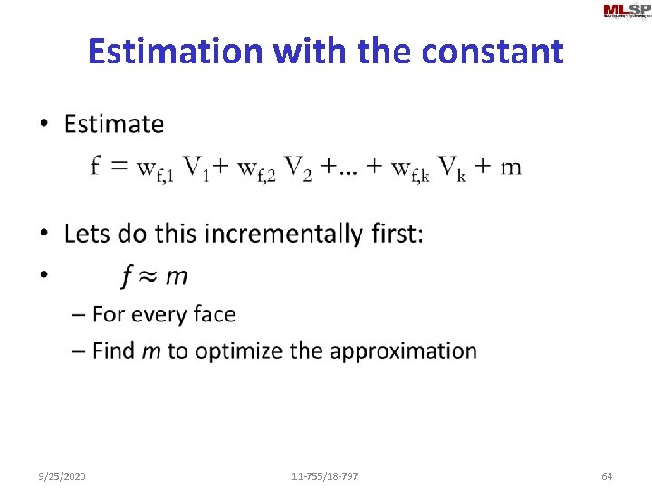
Estimation with the constant • 9/25/2020 11 -755/18 -797 64

Estimation with the constant • 9/25/2020 11 -755/18 -797 65

Estimation the remaining • 9/25/2020 11 -755/18 -797 66

Estimating the Affine model • 9/25/2020 11 -755/18 -797 67

Estimating the Affine model • 9/25/2020 11 -755/18 -797 68

Properties of the affine model • 9/25/2020 11 -755/18 -797 69

Linear vs. Affine • The model we saw – Approximate every face f as f = wf, 1 V 1+ wf, 2 V 2 +. . . + wf, k Vk – The Karhunen Loeve Transform – Retains maximum Energy for any order k • If you add a constant f = wf, 1 V 1+ wf, 2 V 2 +. . . + wf, k Vk + m – Principal Component Analysis – Retains maximum Variance for any order k 9/25/2020 11 -755/18 -797 70

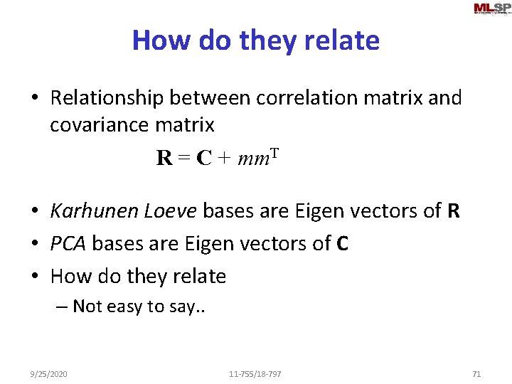
How do they relate • Relationship between correlation matrix and covariance matrix R = C + mm. T • Karhunen Loeve bases are Eigen vectors of R • PCA bases are Eigen vectors of C • How do they relate – Not easy to say. . 9/25/2020 11 -755/18 -797 71

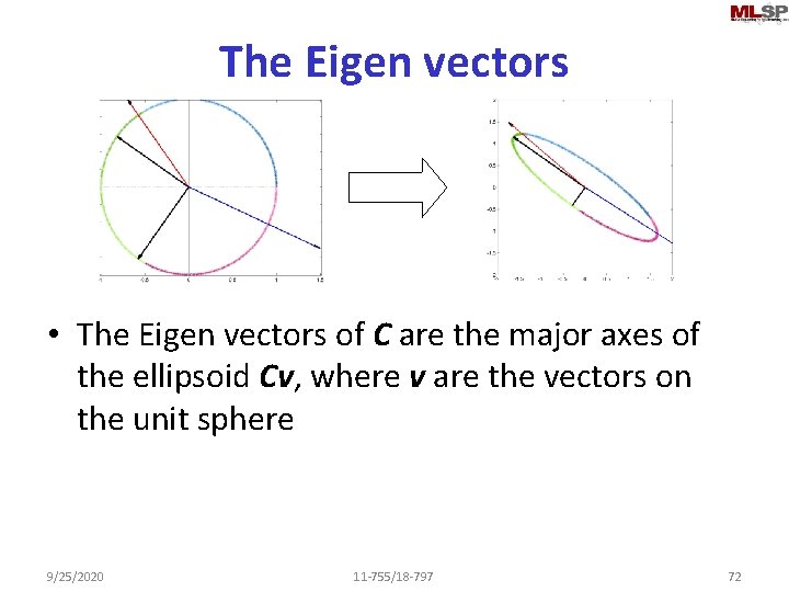
The Eigen vectors • The Eigen vectors of C are the major axes of the ellipsoid Cv, where v are the vectors on the unit sphere 9/25/2020 11 -755/18 -797 72

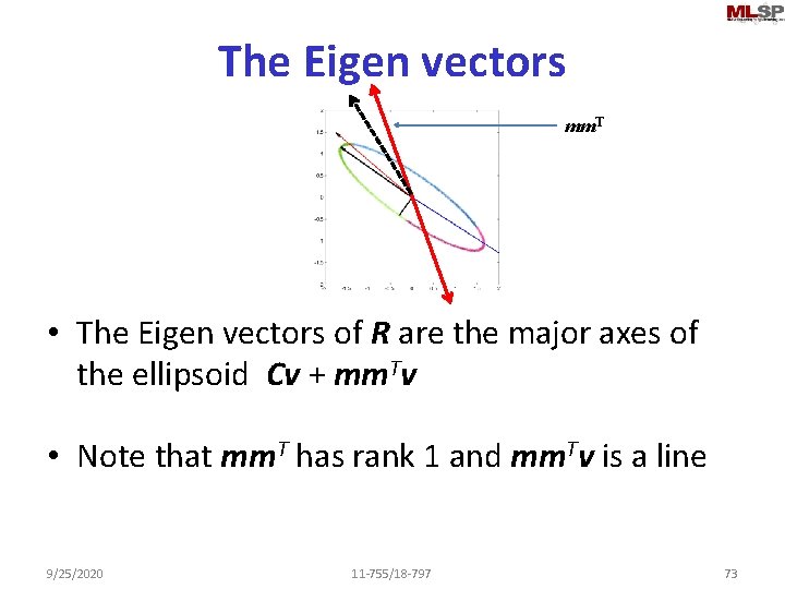
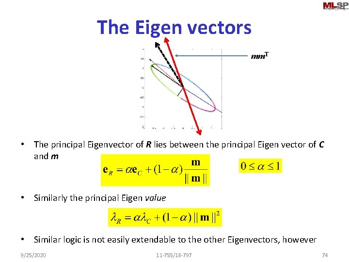
The Eigen vectors mm. T • The Eigen vectors of R are the major axes of the ellipsoid Cv + mm. Tv • Note that mm. T has rank 1 and mm. Tv is a line 9/25/2020 11 -755/18 -797 73

The Eigen vectors mm. T • The principal Eigenvector of R lies between the principal Eigen vector of C and m • Similarly the principal Eigen value • Similar logic is not easily extendable to the other Eigenvectors, however 9/25/2020 11 -755/18 -797 74

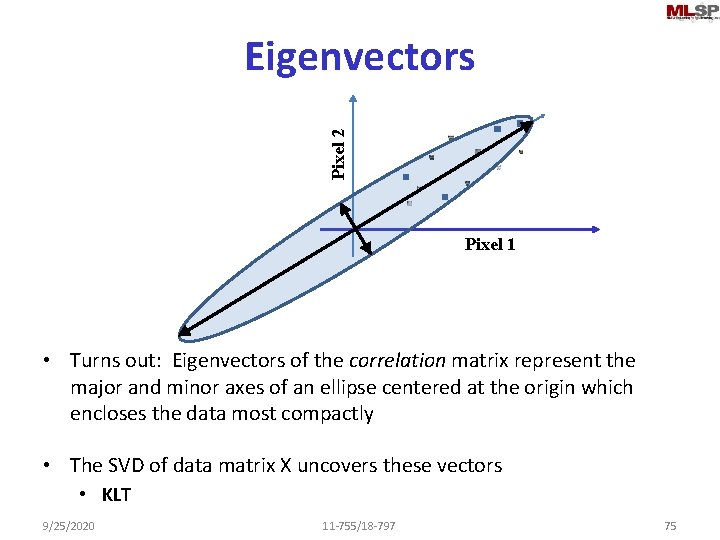
Pixel 2 Eigenvectors Pixel 1 • Turns out: Eigenvectors of the correlation matrix represent the major and minor axes of an ellipse centered at the origin which encloses the data most compactly • The SVD of data matrix X uncovers these vectors • KLT 9/25/2020 11 -755/18 -797 75

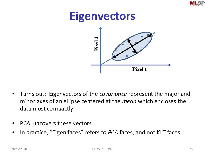
Pixel 2 Eigenvectors Pixel 1 • Turns out: Eigenvectors of the covariance represent the major and minor axes of an ellipse centered at the mean which encloses the data most compactly • PCA uncovers these vectors • In practice, “Eigen faces” refers to PCA faces, and not KLT faces 9/25/2020 11 -755/18 -797 76

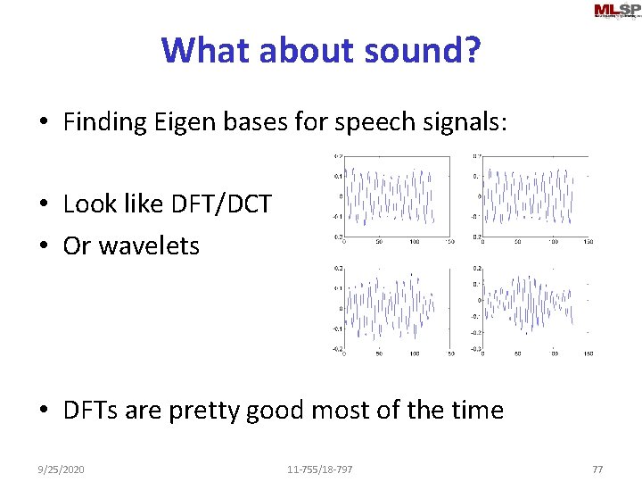
What about sound? • Finding Eigen bases for speech signals: • Look like DFT/DCT • Or wavelets • DFTs are pretty good most of the time 9/25/2020 11 -755/18 -797 77

Eigen Analysis • Can often find surprising features in your data • Trends, relationships, more • Commonly used in recommender systems • An interesting example. . 9/25/2020 11 -755/18 -797 78

Eigen Analysis • Cheng Liu’s research on pipes. . • SVD automatically separates useful and uninformative features 9/25/2020 11 -755/18 -797 79

Eigen Analysis • But for all of this, we need to “preprocess” data • Eliminate unnecessary aspects – E. g. noise, other externally caused variations. . 9/25/2020 11 -755/18 -797 80