Machine Learning for Signal Processing Principal Component Analysis

Machine Learning for Signal Processing Principal Component Analysis & Independent Component Analysis Class 8. 24 Feb 2015 Instructor: Bhiksha Raj 10/2/2020 11755/18797 1

Recall: Representing images • The most common element in the image: background – Or rather large regions of relatively featureless shading – Uniform sequences of numbers 10/2/2020 11 -755/18 -797 2

“Bases” B 1 B 2 B 3 B 4 B 5 B 6 • “Bases” are the “standard” units such that all instances can be expressed a weighted combinations of these units • Ideal requirements: Bases must be orthogonal • Checkerboards are one choice of bases – Orthogonal – But not “smooth” • Other choices of bases: Complex exponentials, Wavelets, etc. . 10/2/2020 11 -755/18 -797 3

Recap: Data specific bases? – Checkerboards, Complex exponentials, Wavelets are data agnostic. . – We use the same bases regardless of the data we analyze • Image of face vs. Image of a forest • Segment of speech vs. Seismic rumble • How about data specific bases – Bases that consider the underlying data • E. g. is there something better than checkerboards to describe faces • Something better than complex exponentials to describe music? 10/2/2020 11 -755/18 -797 4

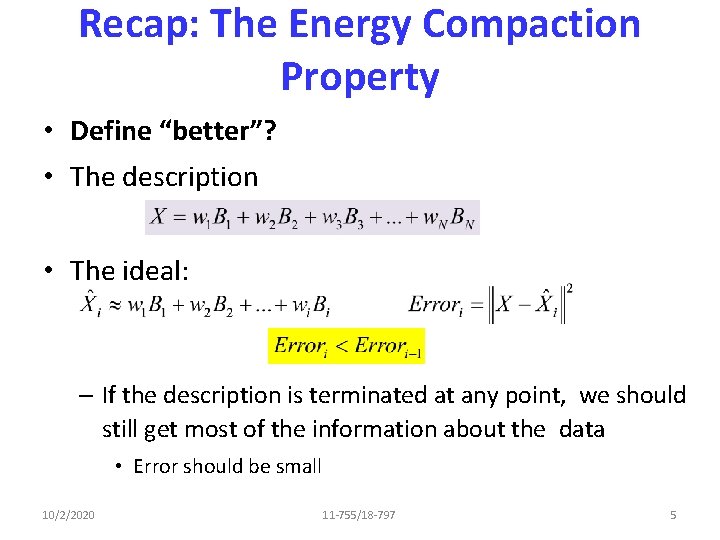
Recap: The Energy Compaction Property • Define “better”? • The description • The ideal: – If the description is terminated at any point, we should still get most of the information about the data • Error should be small 10/2/2020 11 -755/18 -797 5

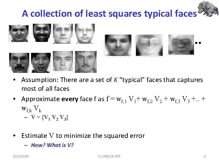
A collection of least squares typical faces • Assumption: There a set of K “typical” faces that captures most of all faces • Approximate every face f as f = wf, 1 V 1+ wf, 2 V 2 + wf, 3 V 3 +. . + wf, k Vk – V = [V 1 V 2 V 3] • Estimate V to minimize the squared error – How? What is V? 10/2/2020 11 -755/18 -797 6

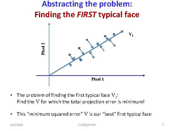
Abstracting the problem: Finding the FIRST typical face Pixel 2 V 1 Pixel 1 • The problem of finding the first typical face V 1: Find the V for which the total projection error is minimum! • This “minimum squared error” V is our “best” first typical face 10/2/2020 11 -755/18 -797 7

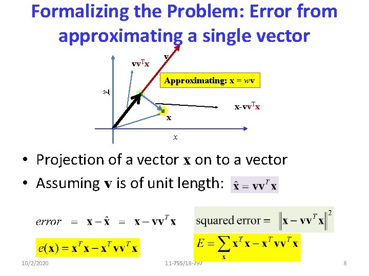
Formalizing the Problem: Error from approximating a single vector vv. Tx v y Approximating: x = wv x-vv. Tx x x • Projection of a vector x on to a vector • Assuming v is of unit length: 10/2/2020 11 -755/18 -797 8

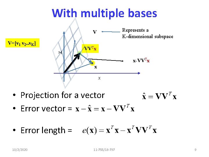
With multiple bases Represents a K-dimensional subspace V y V=[v 1 v 2. . v. K] VVTx x-VVTx x x • Projection for a vector • Error vector = • Error length = 10/2/2020 11 -755/18 -797 9

With multiple bases V y V=[v 1 v 2. . v. K] x • Error for one vector: • Error for many vectors • Goal: Estimate V to minimize this error! 10/2/2020 11 -755/18 -797 10

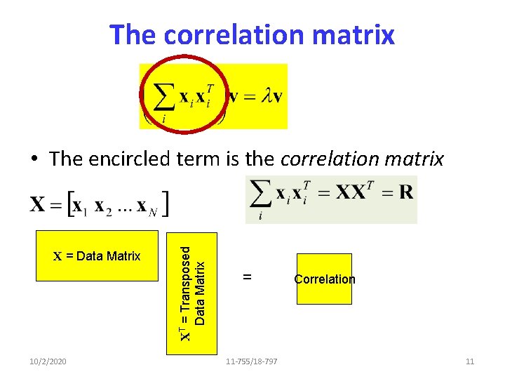
The correlation matrix X = Data Matrix 10/2/2020 XT = Transposed Data Matrix • The encircled term is the correlation matrix = 11 -755/18 -797 Correlation 11

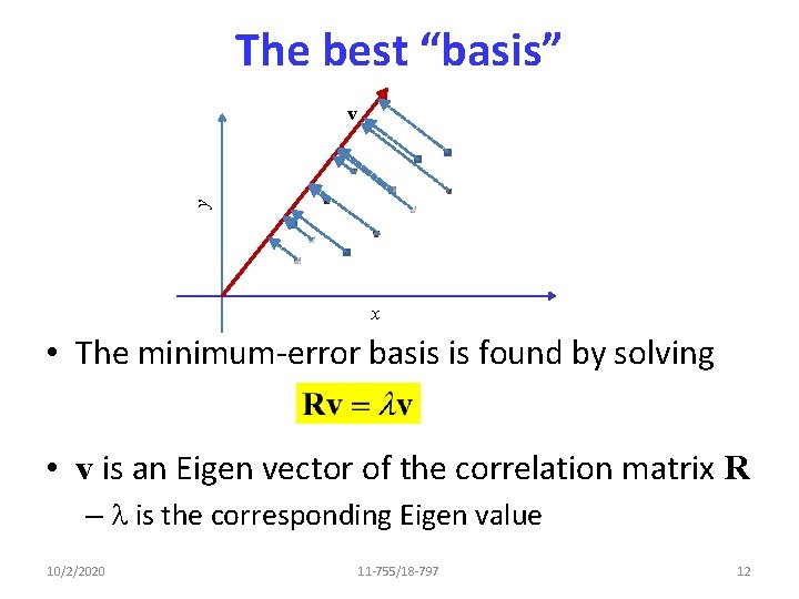
The best “basis” y v x • The minimum-error basis is found by solving • v is an Eigen vector of the correlation matrix R – l is the corresponding Eigen value 10/2/2020 11 -755/18 -797 12

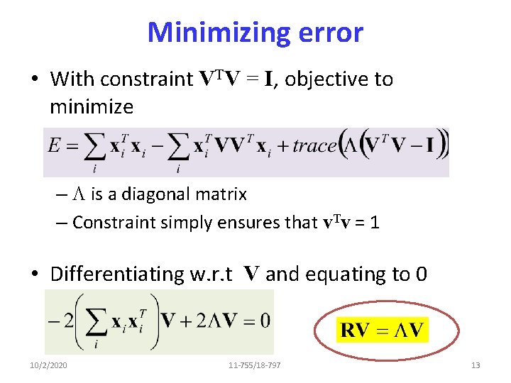
Minimizing error • With constraint VTV = I, objective to minimize – L is a diagonal matrix – Constraint simply ensures that v. Tv = 1 • Differentiating w. r. t V and equating to 0 10/2/2020 11 -755/18 -797 13

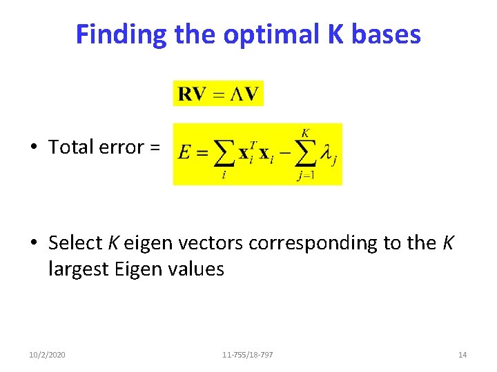
Finding the optimal K bases • Total error = • Select K eigen vectors corresponding to the K largest Eigen values 10/2/2020 11 -755/18 -797 14

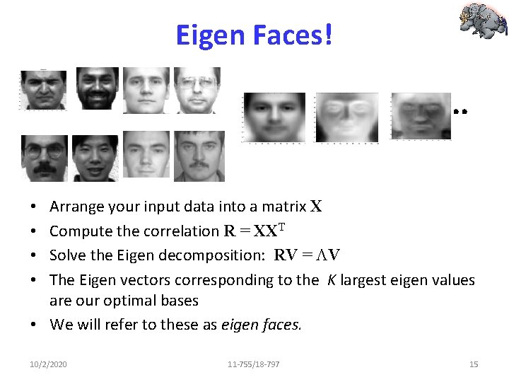
Eigen Faces! Arrange your input data into a matrix X Compute the correlation R = XXT Solve the Eigen decomposition: RV = LV The Eigen vectors corresponding to the K largest eigen values are our optimal bases • We will refer to these as eigen faces. • • 10/2/2020 11 -755/18 -797 15

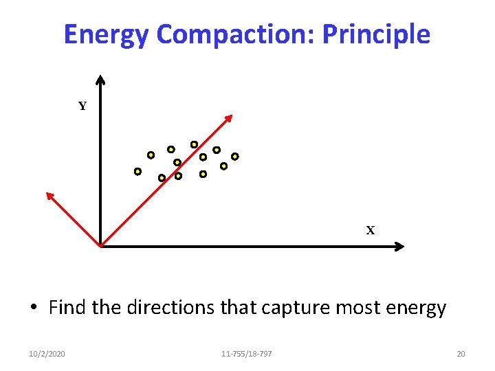
Energy Compaction: Principle Y X • Find the directions that capture most energy 10/2/2020 11 -755/18 -797 20

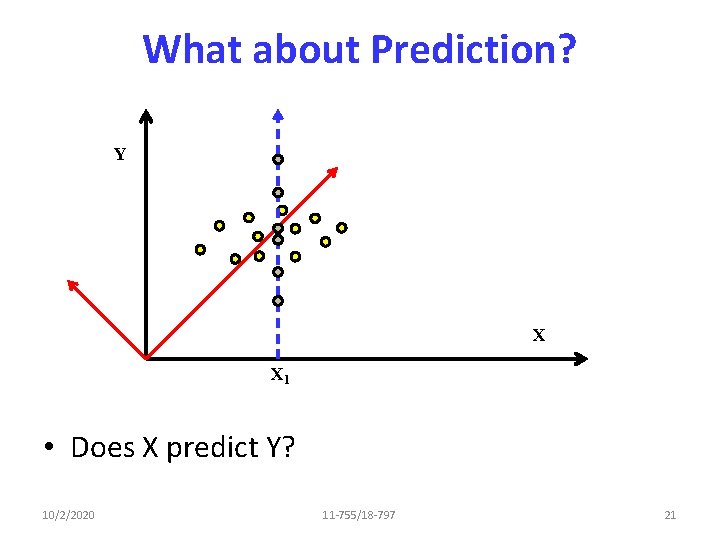
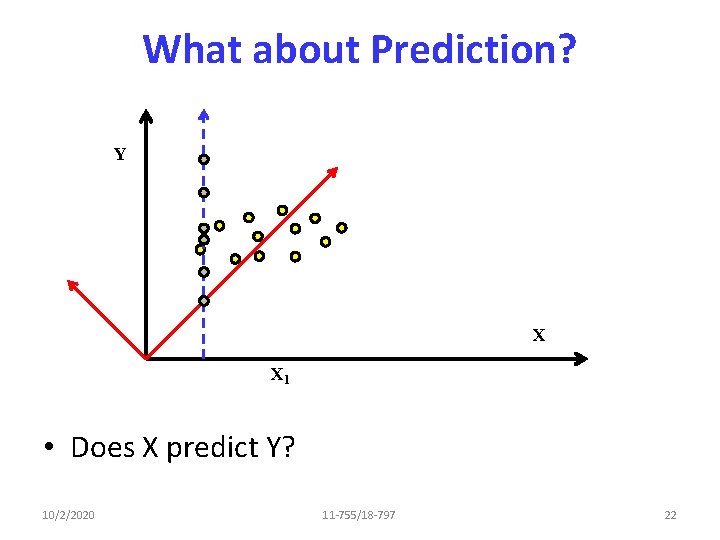
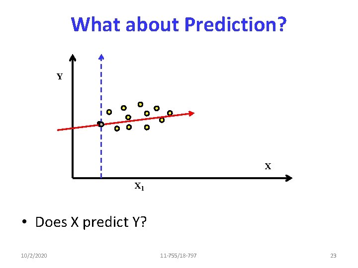
What about Prediction? Y X X 1 • Does X predict Y? 10/2/2020 11 -755/18 -797 21

What about Prediction? Y X X 1 • Does X predict Y? 10/2/2020 11 -755/18 -797 22

What about Prediction? Y X X 1 • Does X predict Y? 10/2/2020 11 -755/18 -797 23

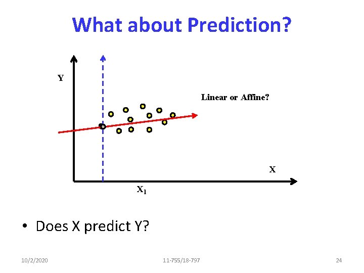
What about Prediction? Y Linear or Affine? X X 1 • Does X predict Y? 10/2/2020 11 -755/18 -797 24

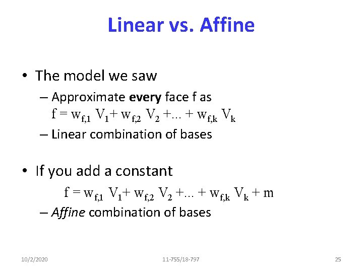
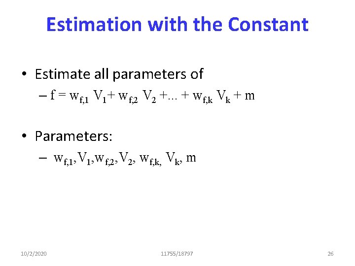
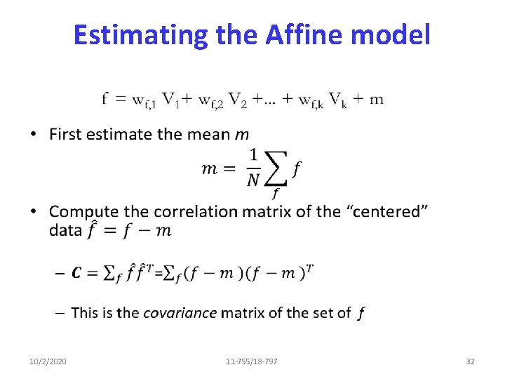
Linear vs. Affine • The model we saw – Approximate every face f as f = wf, 1 V 1+ wf, 2 V 2 +. . . + wf, k Vk – Linear combination of bases • If you add a constant f = wf, 1 V 1+ wf, 2 V 2 +. . . + wf, k Vk + m – Affine combination of bases 10/2/2020 11 -755/18 -797 25

Estimation with the Constant • Estimate all parameters of – f = wf, 1 V 1+ wf, 2 V 2 +. . . + wf, k Vk + m • Parameters: – wf, 1, V 1, wf, 2, V 2, wf, k, Vk, m 10/2/2020 11755/18797 26

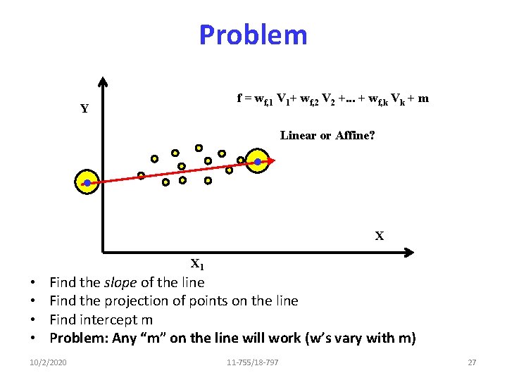
Problem f = wf, 1 V 1+ wf, 2 V 2 +. . . + wf, k Vk + m Y Linear or Affine? X X 1 • • Find the slope of the line Find the projection of points on the line Find intercept m Problem: Any “m” on the line will work (w’s vary with m) 10/2/2020 11 -755/18 -797 27

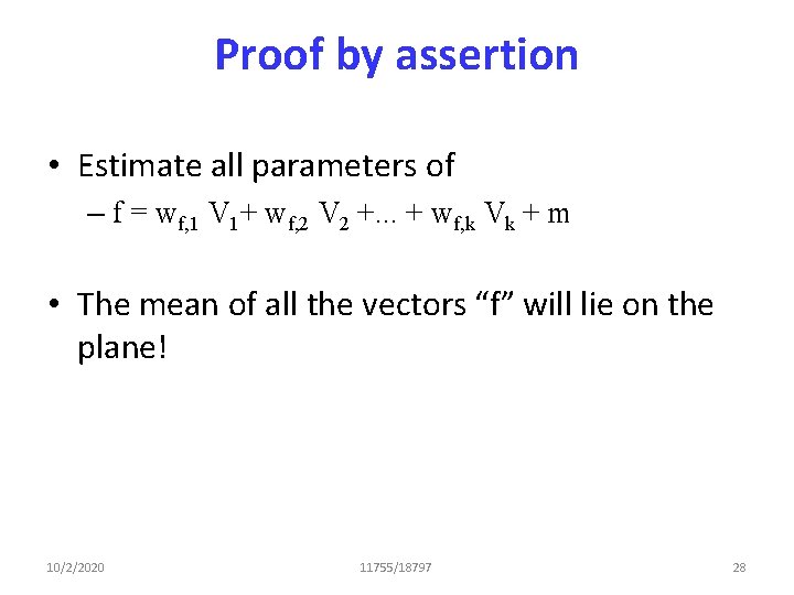
Proof by assertion • Estimate all parameters of – f = wf, 1 V 1+ wf, 2 V 2 +. . . + wf, k Vk + m • The mean of all the vectors “f” will lie on the plane! 10/2/2020 11755/18797 28

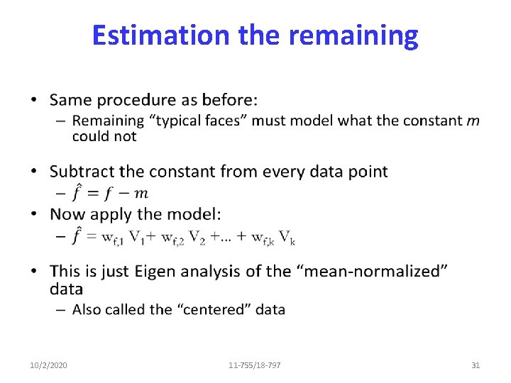
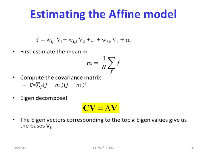
Estimation the remaining • 10/2/2020 11 -755/18 -797 31

Estimating the Affine model • 10/2/2020 11 -755/18 -797 32

Estimating the Affine model • 10/2/2020 11 -755/18 -797 33

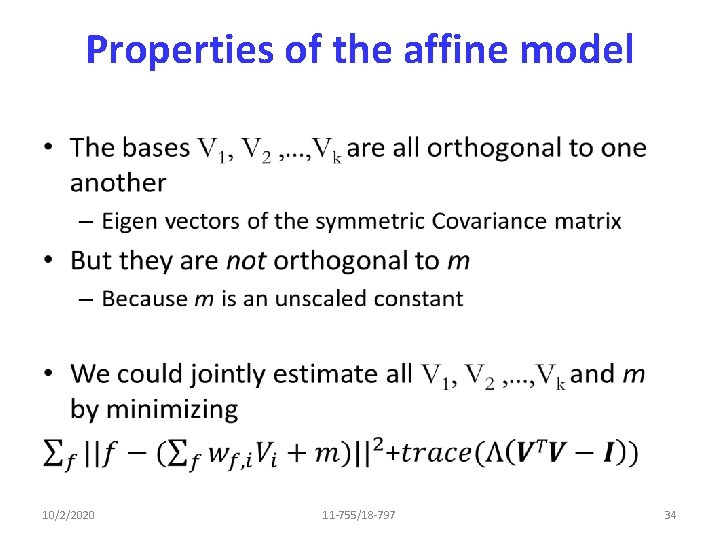
Properties of the affine model • 10/2/2020 11 -755/18 -797 34

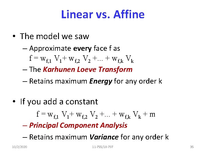
Linear vs. Affine • The model we saw – Approximate every face f as f = wf, 1 V 1+ wf, 2 V 2 +. . . + wf, k Vk – The Karhunen Loeve Transform – Retains maximum Energy for any order k • If you add a constant f = wf, 1 V 1+ wf, 2 V 2 +. . . + wf, k Vk + m – Principal Component Analysis – Retains maximum Variance for any order k 10/2/2020 11 -755/18 -797 35

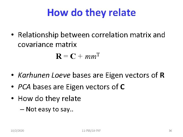
How do they relate • Relationship between correlation matrix and covariance matrix R = C + mm. T • Karhunen Loeve bases are Eigen vectors of R • PCA bases are Eigen vectors of C • How do they relate – Not easy to say. . 10/2/2020 11 -755/18 -797 36

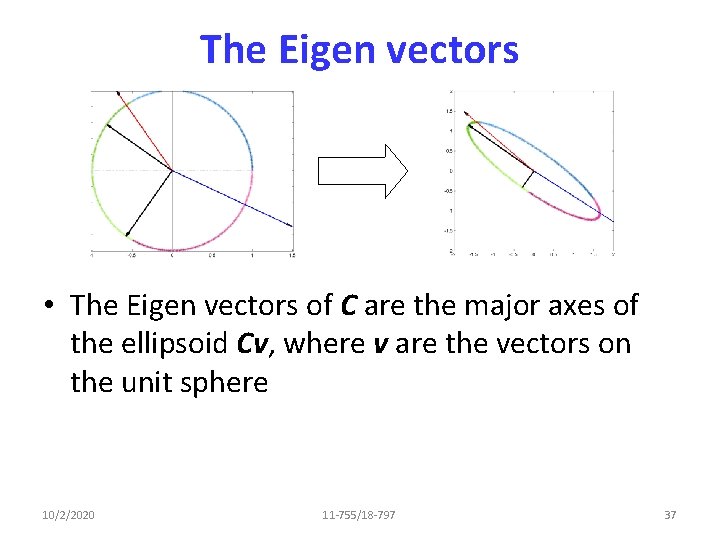
The Eigen vectors • The Eigen vectors of C are the major axes of the ellipsoid Cv, where v are the vectors on the unit sphere 10/2/2020 11 -755/18 -797 37

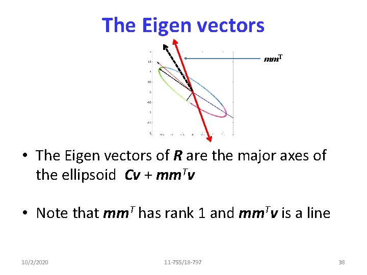
The Eigen vectors mm. T • The Eigen vectors of R are the major axes of the ellipsoid Cv + mm. Tv • Note that mm. T has rank 1 and mm. Tv is a line 10/2/2020 11 -755/18 -797 38

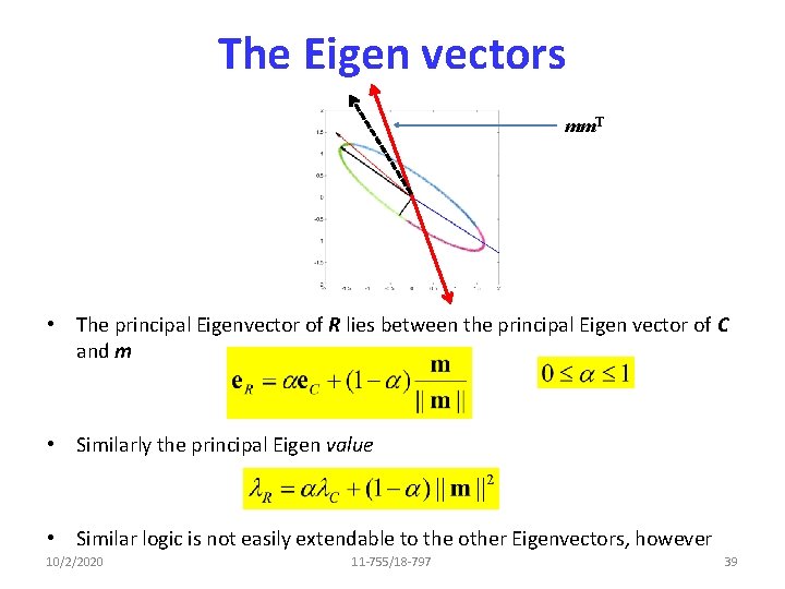
The Eigen vectors mm. T • The principal Eigenvector of R lies between the principal Eigen vector of C and m • Similarly the principal Eigen value • Similar logic is not easily extendable to the other Eigenvectors, however 10/2/2020 11 -755/18 -797 39

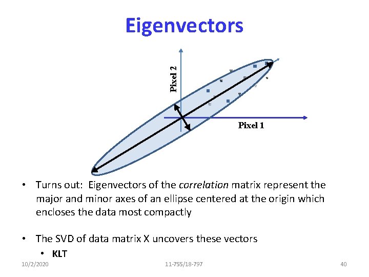
Pixel 2 Eigenvectors Pixel 1 • Turns out: Eigenvectors of the correlation matrix represent the major and minor axes of an ellipse centered at the origin which encloses the data most compactly • The SVD of data matrix X uncovers these vectors • KLT 10/2/2020 11 -755/18 -797 40

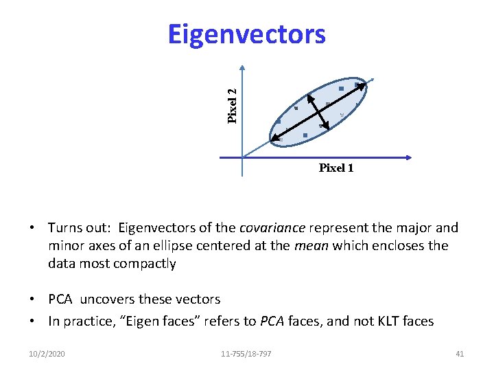
Pixel 2 Eigenvectors Pixel 1 • Turns out: Eigenvectors of the covariance represent the major and minor axes of an ellipse centered at the mean which encloses the data most compactly • PCA uncovers these vectors • In practice, “Eigen faces” refers to PCA faces, and not KLT faces 10/2/2020 11 -755/18 -797 41

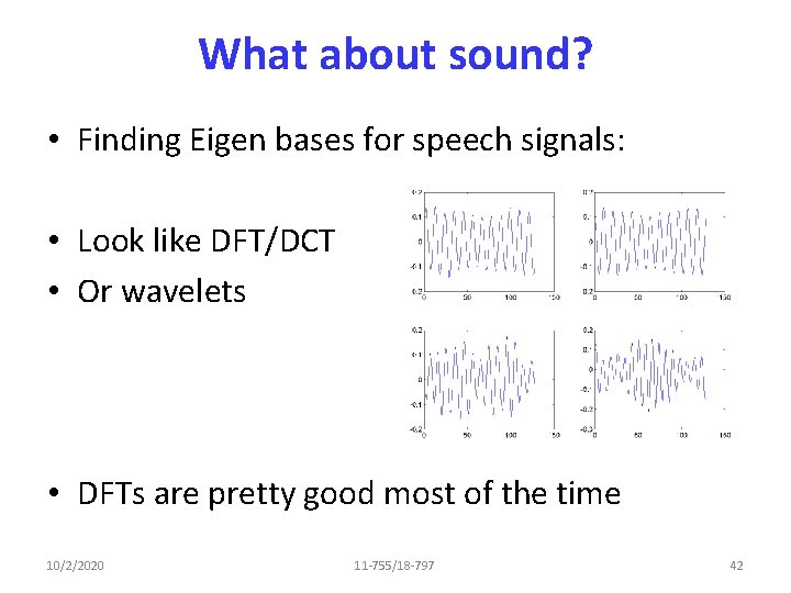
What about sound? • Finding Eigen bases for speech signals: • Look like DFT/DCT • Or wavelets • DFTs are pretty good most of the time 10/2/2020 11 -755/18 -797 42

Eigen Analysis • Can often find surprising features in your data • Trends, relationships, more • Commonly used in recommender systems • An interesting example. . 10/2/2020 11 -755/18 -797 43

Eigen Analysis • Cheng Liu’s research on pipes. . • SVD automatically separates useful and uninformative features 10/2/2020 11 -755/18 -797 44

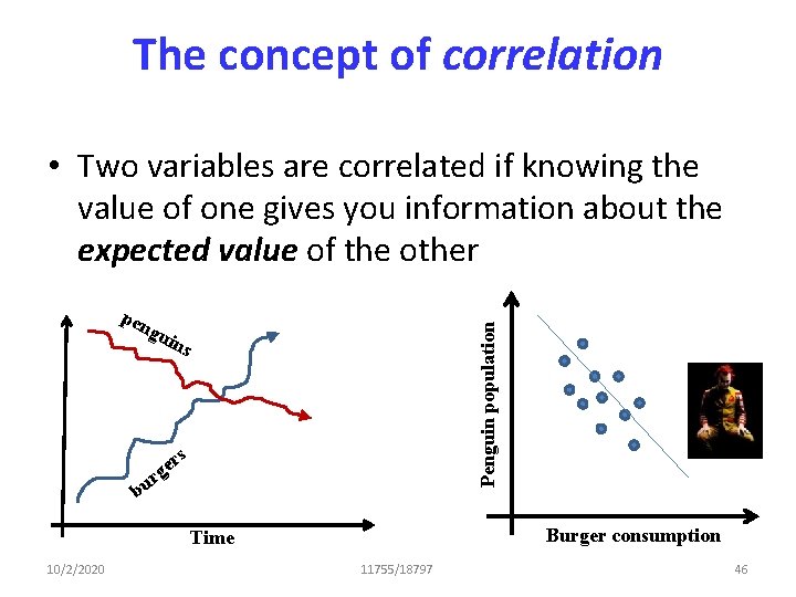
Correlation vs. Causation • The consumption of burgers has gone up steadily in the past decade • In the same period, the penguin population of Antarctica has gone down Correlation, not Causation (unless Mc. Donalds has a top-secret Antarctica division) 10/2/2020 11755/18797 45

The concept of correlation • Two variables are correlated if knowing the value of one gives you information about the expected value of the other pen Penguin population gui ns rs e g ur b Burger consumption Time 10/2/2020 11755/18797 46

The statistical concept of correlatedness • Two variables X and Y are correlated if If knowing X gives you an expected value of Y • X and Y are uncorrelated if knowing X tells you nothing about the expected value of Y – Although it could give you other information – How? 10/2/2020 11755/18797 47

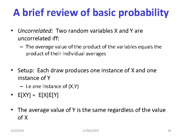
A brief review of basic probability • Uncorrelated: Two random variables X and Y are uncorrelated iff: – The average value of the product of the variables equals the product of their individual averages • Setup: Each draw produces one instance of X and one instance of Y – I. e one instance of (X, Y) • E[XY] = E[X]E[Y] • The average value of Y is the same regardless of the value of X 10/2/2020 11755/18797 48

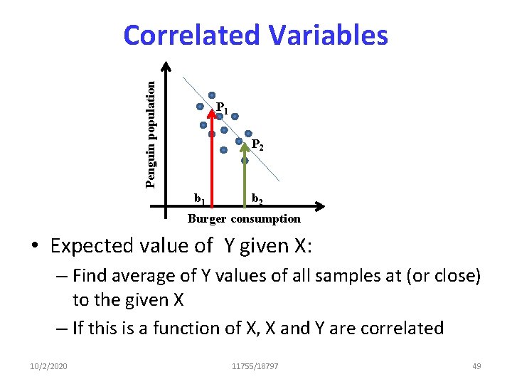
Penguin population Correlated Variables P 1 P 2 b 1 b 2 Burger consumption • Expected value of Y given X: – Find average of Y values of all samples at (or close) to the given X – If this is a function of X, X and Y are correlated 10/2/2020 11755/18797 49

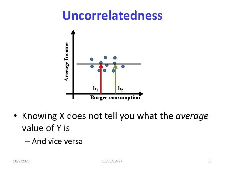
Average Income Uncorrelatedness b 1 b 2 Burger consumption • Knowing X does not tell you what the average value of Y is – And vice versa 10/2/2020 11755/18797 50

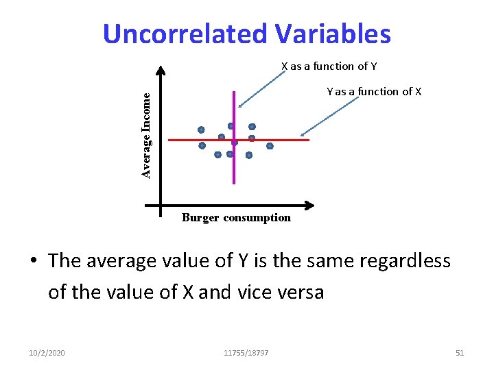
Uncorrelated Variables X as a function of Y Average Income Y as a function of X Burger consumption • The average value of Y is the same regardless of the value of X and vice versa 10/2/2020 11755/18797 51

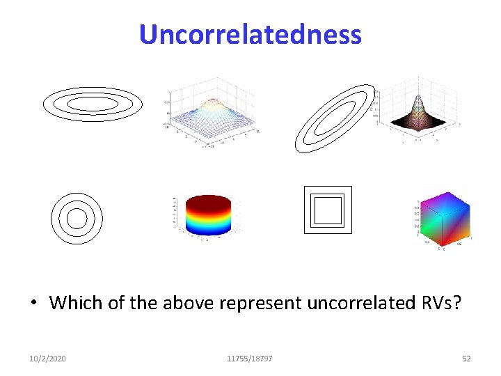
Uncorrelatedness • Which of the above represent uncorrelated RVs? 10/2/2020 11755/18797 52

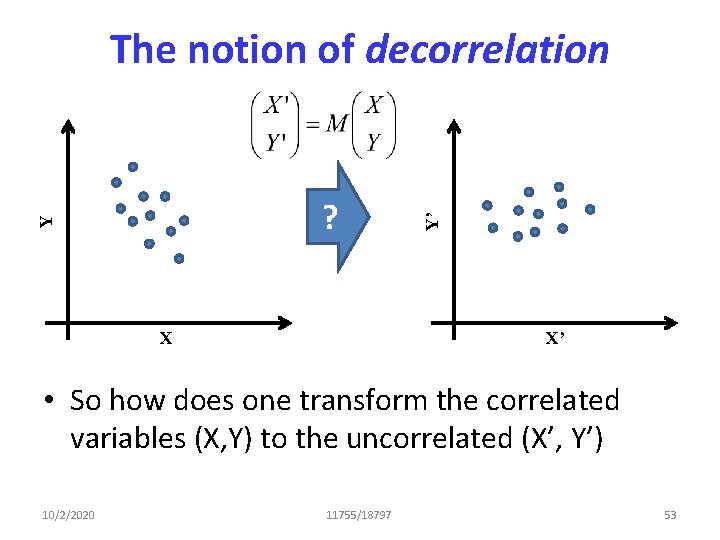
Y ? X Y’ The notion of decorrelation X’ • So how does one transform the correlated variables (X, Y) to the uncorrelated (X’, Y’) 10/2/2020 11755/18797 53

What does “uncorrelated” mean Assuming 0 mean Y’ 0 • • E[X’] = constant (0) E[Y’] = constant (0) E[X’|Y’] = 0 E[X’Y’] = EY’[E [X’|Y’]] = 0 X’ • If Y is a matrix of vectors, YYT = diagonal 10/2/2020 11755/18797 54

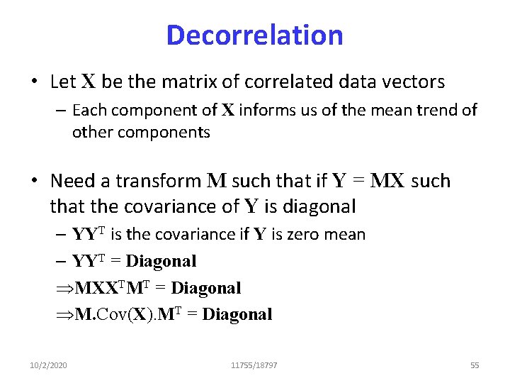
Decorrelation • Let X be the matrix of correlated data vectors – Each component of X informs us of the mean trend of other components • Need a transform M such that if Y = MX such that the covariance of Y is diagonal – YYT is the covariance if Y is zero mean – YYT = Diagonal ÞMXXTMT = Diagonal ÞM. Cov(X). MT = Diagonal 10/2/2020 11755/18797 55

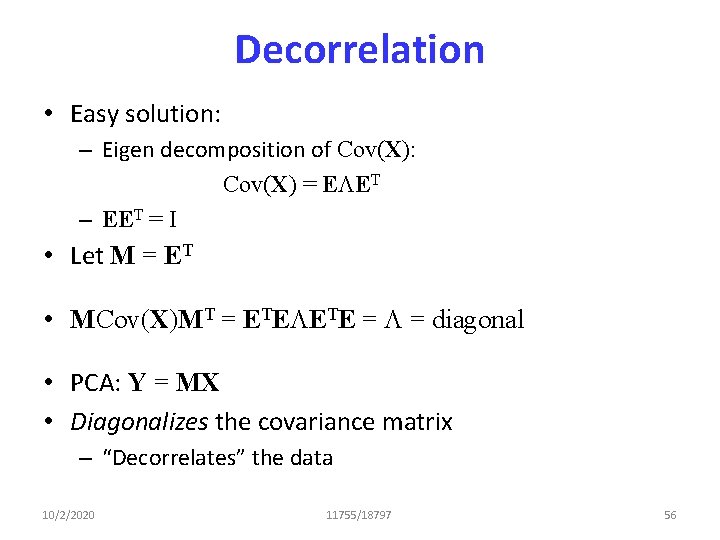
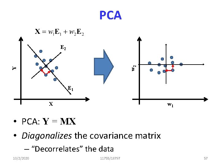
Decorrelation • Easy solution: – Eigen decomposition of Cov(X): Cov(X) = ELET – EET = I • Let M = ET • MCov(X)MT = ETELETE = L = diagonal • PCA: Y = MX • Diagonalizes the covariance matrix – “Decorrelates” the data 10/2/2020 11755/18797 56

PCA Y w 2 E 1 X w 1 • PCA: Y = MX • Diagonalizes the covariance matrix – “Decorrelates” the data 10/2/2020 11755/18797 57

The statistical concept of Independence • Two variables X and Y are dependent if If knowing X gives you any information about Y • X and Y are independent if knowing X tells you nothing at all of Y 10/2/2020 11755/18797 58

A brief review of basic probability • Independence: Two random variables X and Y are independent iff: – Their joint probability equals the product of their individual probabilities • P(X, Y) = P(X)P(Y) • Independence implies uncorrelatedness – The average value of X is the same regardless of the value of Y • E[X|Y] = E[X] – But not the other way 10/2/2020 11755/18797 59

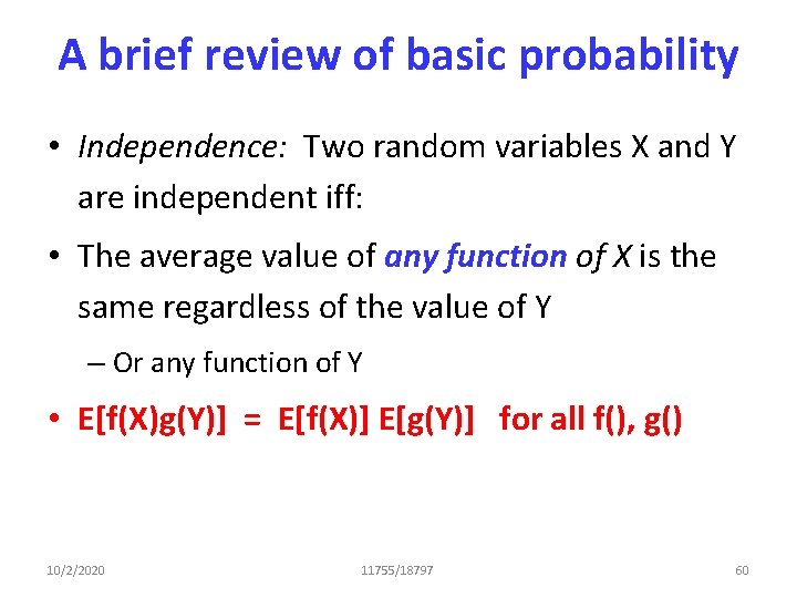
A brief review of basic probability • Independence: Two random variables X and Y are independent iff: • The average value of any function of X is the same regardless of the value of Y – Or any function of Y • E[f(X)g(Y)] = E[f(X)] E[g(Y)] for all f(), g() 10/2/2020 11755/18797 60

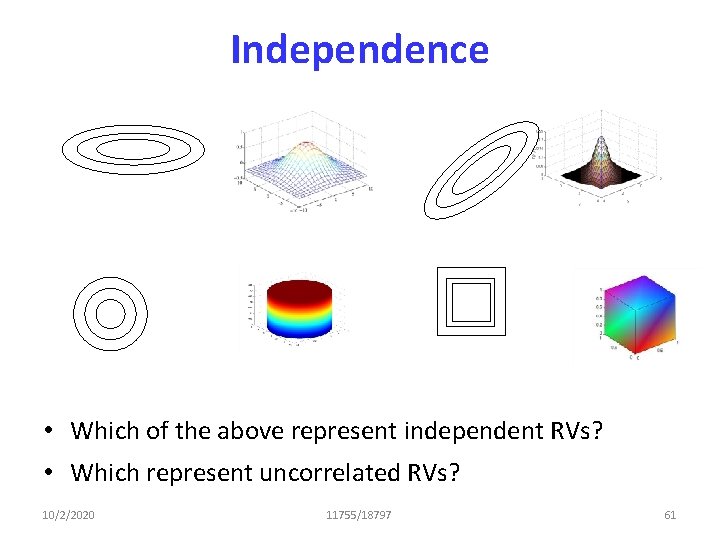
Independence • Which of the above represent independent RVs? • Which represent uncorrelated RVs? 10/2/2020 11755/18797 61

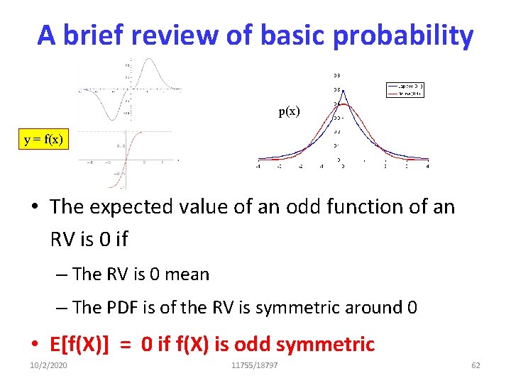
A brief review of basic probability p(x) y = f(x) • The expected value of an odd function of an RV is 0 if – The RV is 0 mean – The PDF is of the RV is symmetric around 0 • E[f(X)] = 0 if f(X) is odd symmetric 10/2/2020 11755/18797 62

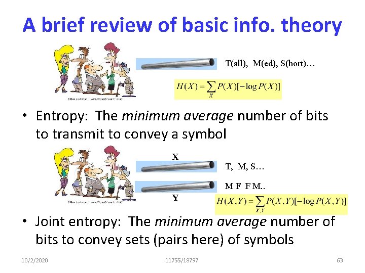
A brief review of basic info. theory T(all), M(ed), S(hort)… • Entropy: The minimum average number of bits to transmit to convey a symbol X T, M, S… M F F M. . Y • Joint entropy: The minimum average number of bits to convey sets (pairs here) of symbols 10/2/2020 11755/18797 63

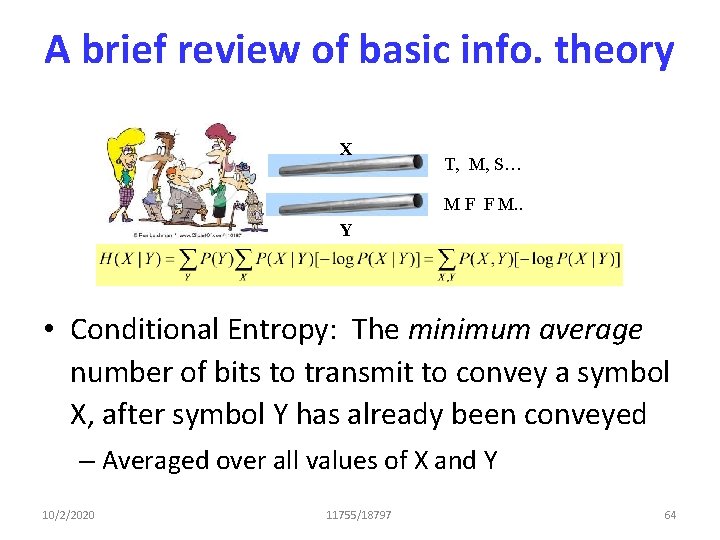
A brief review of basic info. theory X T, M, S… M F F M. . Y • Conditional Entropy: The minimum average number of bits to transmit to convey a symbol X, after symbol Y has already been conveyed – Averaged over all values of X and Y 10/2/2020 11755/18797 64

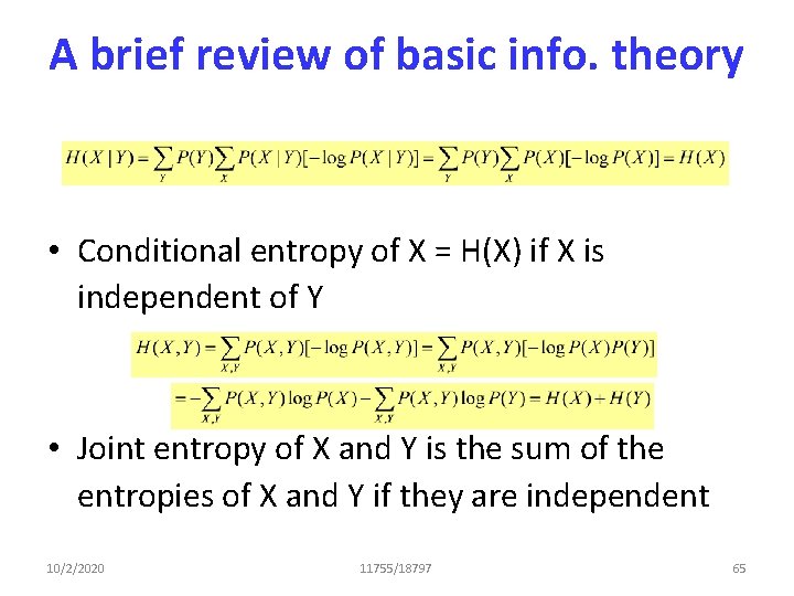
A brief review of basic info. theory • Conditional entropy of X = H(X) if X is independent of Y • Joint entropy of X and Y is the sum of the entropies of X and Y if they are independent 10/2/2020 11755/18797 65

Onward. . 10/2/2020 11755/18797 66

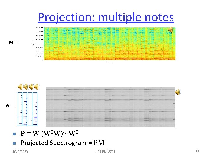
Projection: multiple notes M= W= n n P = W (WTW)-1 WT Projected Spectrogram = PM 10/2/2020 11755/18797 67

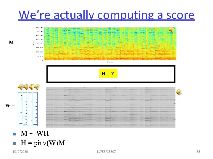
We’re actually computing a score M= H=? W= n n M ~ WH H = pinv(W)M 10/2/2020 11755/18797 68

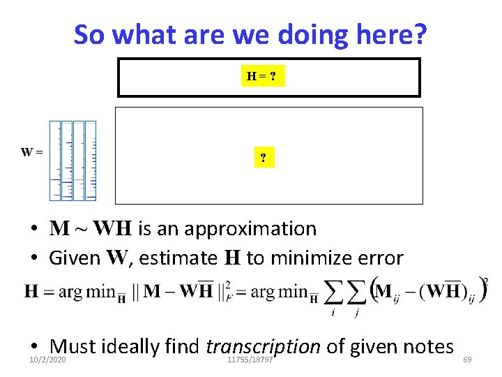
So what are we doing here? H=? W= ? • M ~ WH is an approximation • Given W, estimate H to minimize error • Must ideally find transcription of given notes 10/2/2020 11755/18797 69

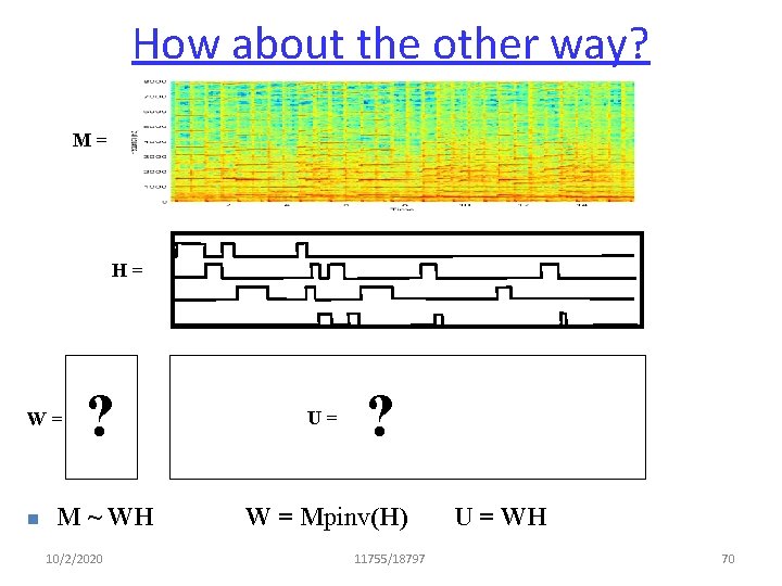
How about the other way? M= H= ? U= M ~ WH W = Mpinv(H) W= n 10/2/2020 ? 11755/18797 U = WH 70

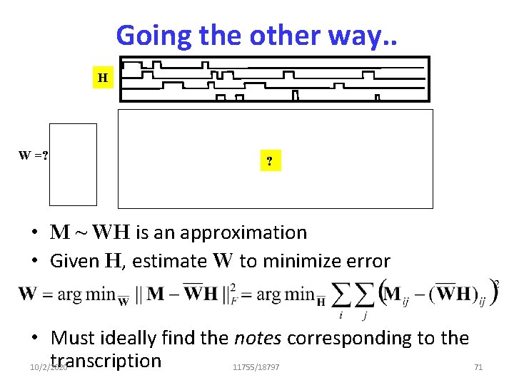
Going the other way. . H W =? ? • M ~ WH is an approximation • Given H, estimate W to minimize error • Must ideally find the notes corresponding to the transcription 10/2/2020 11755/18797 71

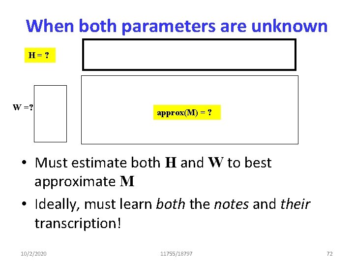
When both parameters are unknown H=? W =? approx(M) = ? • Must estimate both H and W to best approximate M • Ideally, must learn both the notes and their transcription! 10/2/2020 11755/18797 72

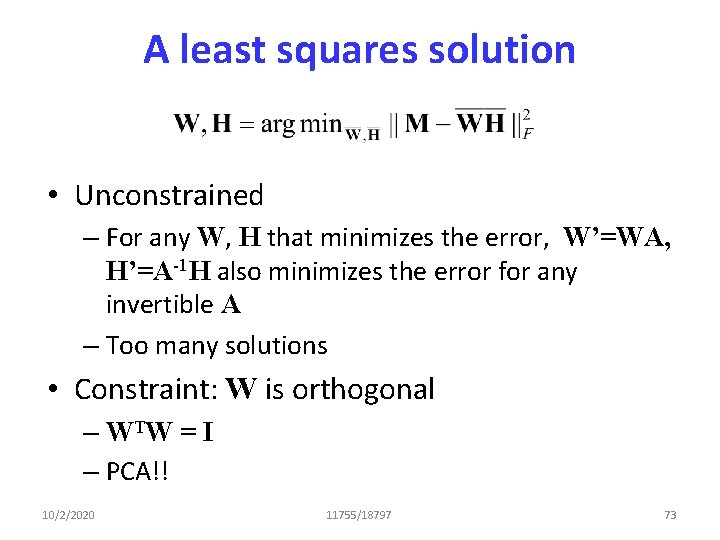
A least squares solution • Unconstrained – For any W, H that minimizes the error, W’=WA, H’=A-1 H also minimizes the error for any invertible A – Too many solutions • Constraint: W is orthogonal – WTW = I – PCA!! 10/2/2020 11755/18797 73

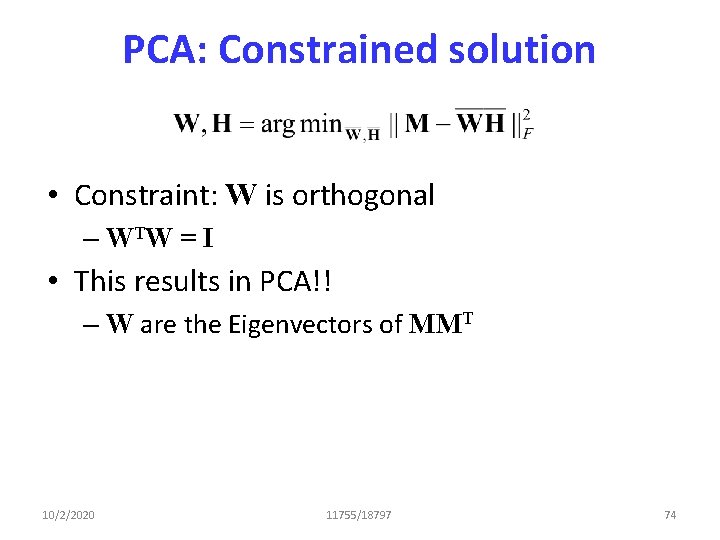
PCA: Constrained solution • Constraint: W is orthogonal – WTW = I • This results in PCA!! – W are the Eigenvectors of MMT 10/2/2020 11755/18797 74

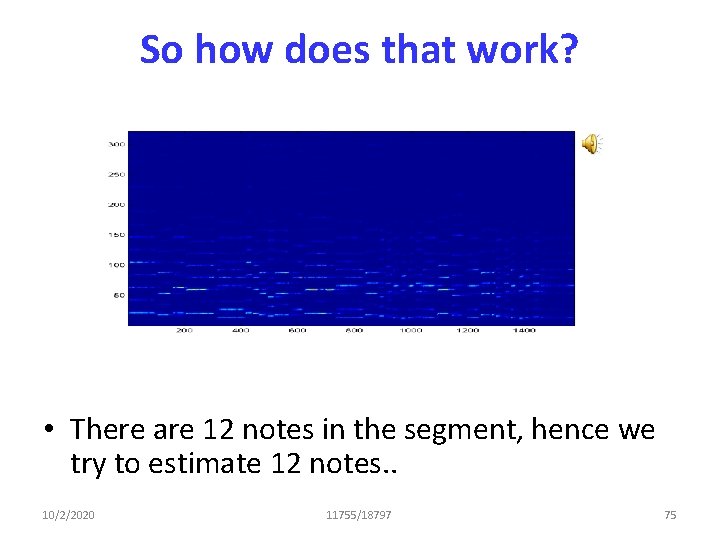
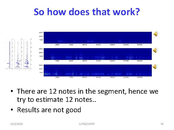
So how does that work? • There are 12 notes in the segment, hence we try to estimate 12 notes. . 10/2/2020 11755/18797 75

So how does that work? • There are 12 notes in the segment, hence we try to estimate 12 notes. . • Results are not good 10/2/2020 11755/18797 76

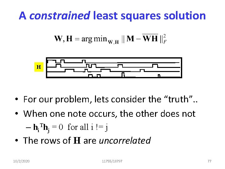
A constrained least squares solution H • For our problem, lets consider the “truth”. . • When one note occurs, the other does not – hi. Thj = 0 for all i != j • The rows of H are uncorrelated 10/2/2020 11755/18797 77

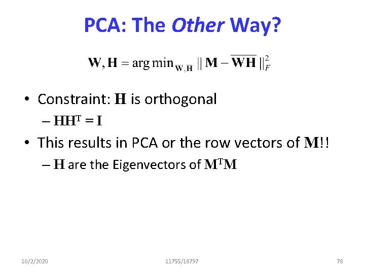
PCA: The Other Way? • Constraint: H is orthogonal – HHT = I • This results in PCA or the row vectors of M!! – H are the Eigenvectors of MTM 10/2/2020 11755/18797 78

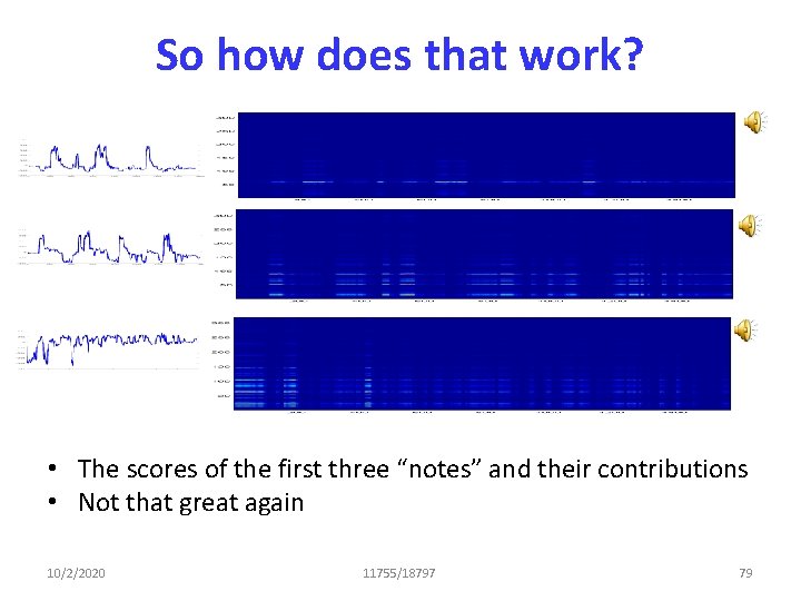
So how does that work? • The scores of the first three “notes” and their contributions • Not that great again 10/2/2020 11755/18797 79

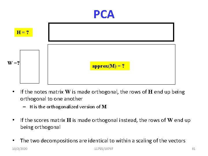
PCA H=? W =? approx(M) = ? • If the notes matrix W is made orthogonal, the rows of H end up being orthogonal to one another – H is the orthogonalized version of M • If the scores matrix H is made orthogonal instead, the rows of W end up being orthogonal • The two decompositions are identical to within a scaling of the vectors 10/2/2020 11755/18797 81

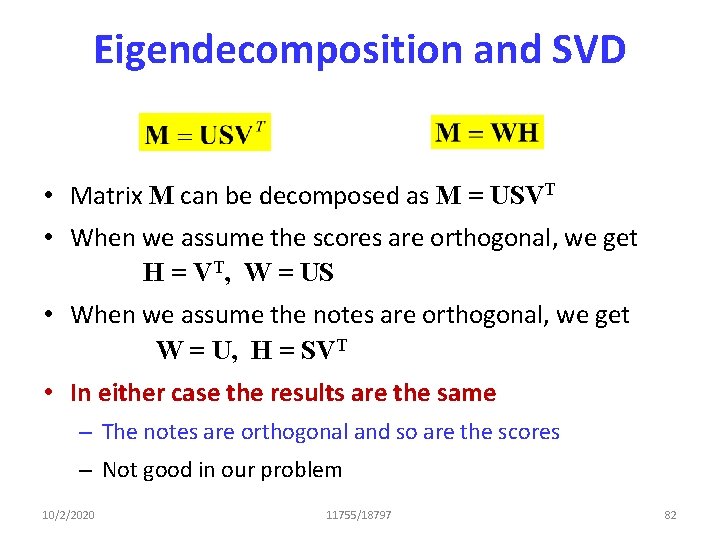
Eigendecomposition and SVD • Matrix M can be decomposed as M = USVT • When we assume the scores are orthogonal, we get H = VT, W = US • When we assume the notes are orthogonal, we get W = U, H = SVT • In either case the results are the same – The notes are orthogonal and so are the scores – Not good in our problem 10/2/2020 11755/18797 82

Orthogonality • In any least-squared error decomposition M=WH, if the columns of W are orthogonal, the rows of H will also be orthogonal • Sometimes mere orthogonality is not enough 10/2/2020 11755/18797 83

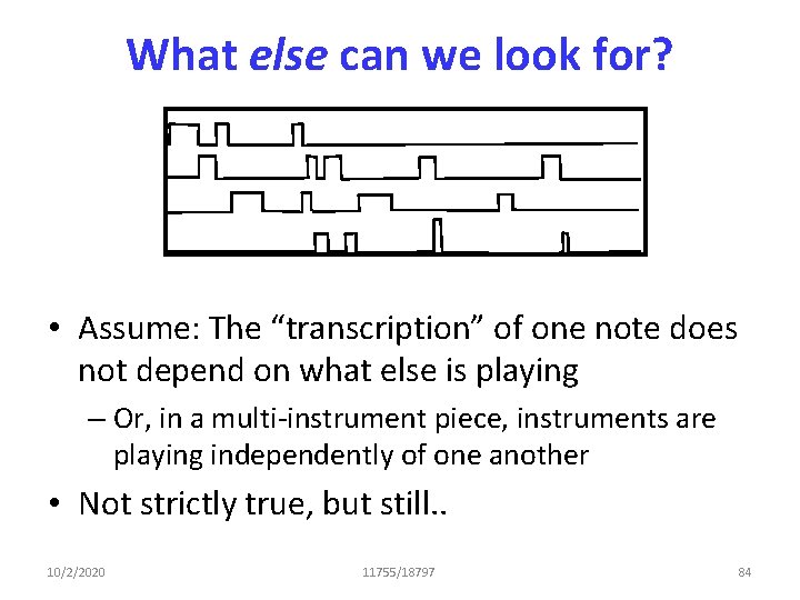
What else can we look for? • Assume: The “transcription” of one note does not depend on what else is playing – Or, in a multi-instrument piece, instruments are playing independently of one another • Not strictly true, but still. . 10/2/2020 11755/18797 84

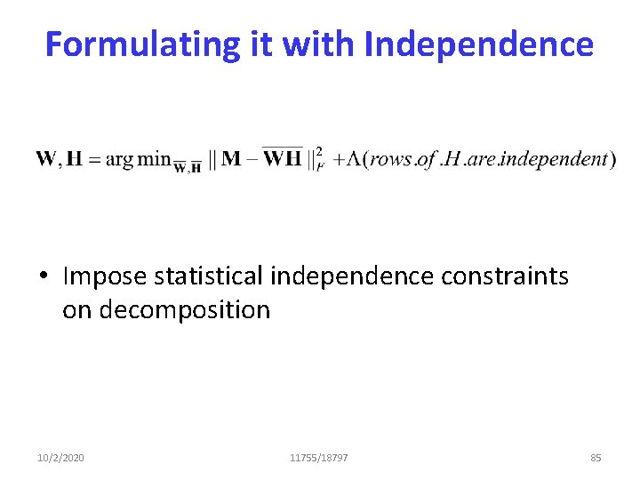
Formulating it with Independence • Impose statistical independence constraints on decomposition 10/2/2020 11755/18797 85

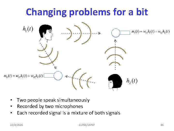
Changing problems for a bit • Two people speak simultaneously • Recorded by two microphones • Each recorded signal is a mixture of both signals 10/2/2020 11755/18797 86

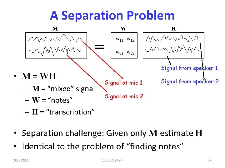
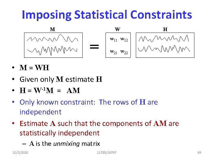
A Separation Problem M W = • M = WH – M = “mixed” signal – W = “notes” – H = “transcription” H w 11 w 12 w 21 w 22 Signal from speaker 1 Signal at mic 1 Signal from speaker 2 Signal at mic 2 • Separation challenge: Given only M estimate H • Identical to the problem of “finding notes” 10/2/2020 11755/18797 87

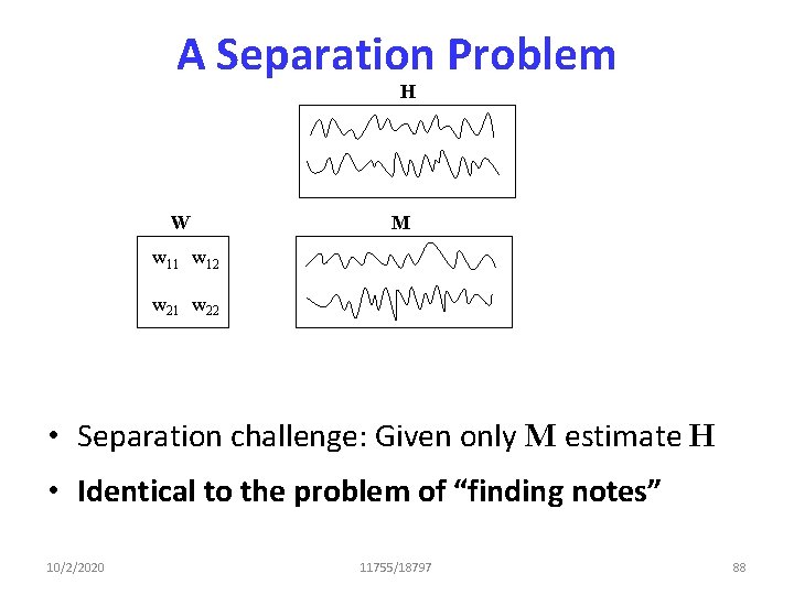
A Separation Problem H W M w 11 w 12 w 21 w 22 • Separation challenge: Given only M estimate H • Identical to the problem of “finding notes” 10/2/2020 11755/18797 88

Imposing Statistical Constraints M W = H w 11 w 12 w 21 w 22 • • M = WH Given only M estimate H H = W-1 M = AM Only known constraint: The rows of H are independent • Estimate A such that the components of AM are statistically independent – A is the unmixing matrix 10/2/2020 11755/18797 89

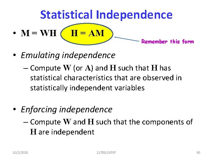
Statistical Independence • M = WH H = AM Remember this form • Emulating independence – Compute W (or A) and H such that H has statistical characteristics that are observed in statistically independent variables • Enforcing independence – Compute W and H such that the components of H are independent 10/2/2020 11755/18797 90

Emulating Independence H • The rows of H are uncorrelated – E[hihj] = E[hi]E[hj] – hi and hj are the ith and jth components of any vector in H • The fourth order moments are independent – – 10/2/2020 E[hihjhkhl] = E[hi]E[hj]E[hk]E[hl] E[hi 2 hjhk] = E[hi 2]E[hj]E[hk] E[hi 2 hj 2] = E[hi 2]E[hj 2] Etc. 11755/18797 91

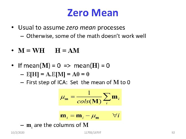
Zero Mean • Usual to assume zero mean processes – Otherwise, some of the math doesn’t work well • M = WH H = AM • If mean(M) = 0 => mean(H) = 0 – E[H] = A. E[M] = A 0 = 0 – First step of ICA: Set the mean of M to 0 – mi are the columns of M 10/2/2020 11755/18797 92

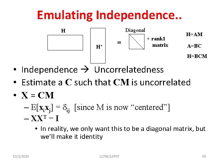
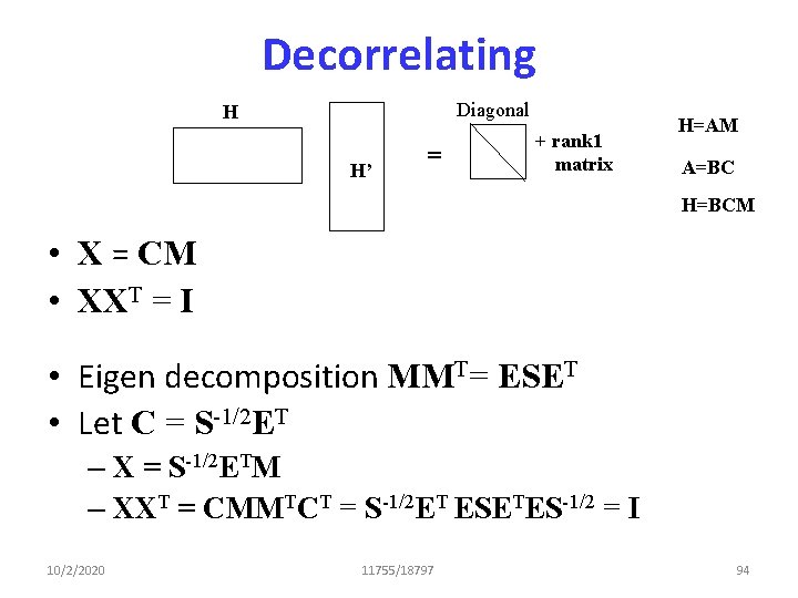
Emulating Independence. . Diagonal H H’ = + rank 1 matrix H=AM A=BC H=BCM • Independence Uncorrelatedness • Estimate a C such that CM is uncorrelated • X = CM – E[xixj] = dij [since M is now “centered”] – XXT = I • In reality, we only want this to be a diagonal matrix, but we’ll make it identity 10/2/2020 11755/18797 93

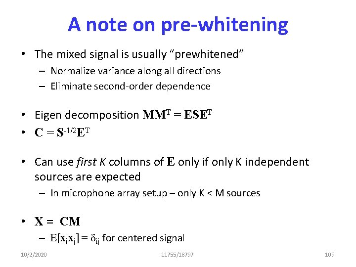
Decorrelating Diagonal H H’ = + rank 1 matrix H=AM A=BC H=BCM • X = CM • XXT = I • Eigen decomposition MMT= ESET • Let C = S-1/2 ET – X = S-1/2 ETM – XXT = CMMTCT = S-1/2 ET ESETES-1/2 = I 10/2/2020 11755/18797 94

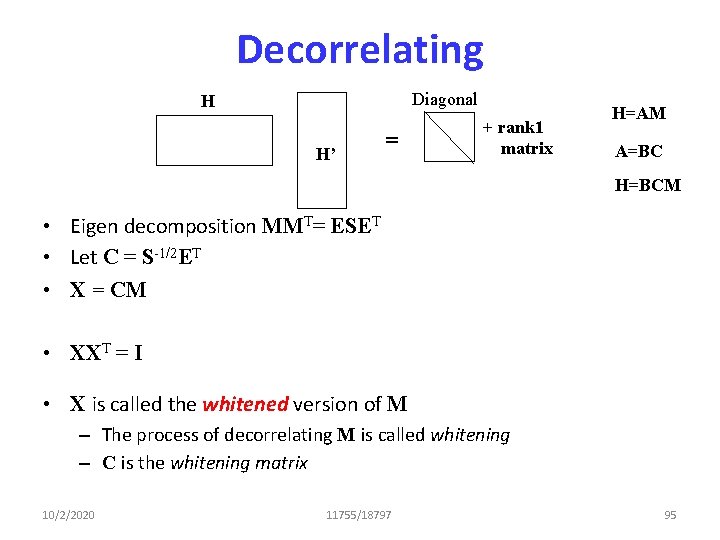
Decorrelating Diagonal H H’ = + rank 1 matrix H=AM A=BC H=BCM • Eigen decomposition MMT= ESET • Let C = S-1/2 ET • X = CM • XXT = I • X is called the whitened version of M – The process of decorrelating M is called whitening – C is the whitening matrix 10/2/2020 11755/18797 95

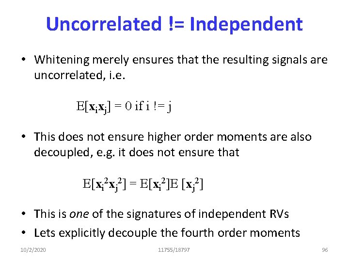
Uncorrelated != Independent • Whitening merely ensures that the resulting signals are uncorrelated, i. e. E[xixj] = 0 if i != j • This does not ensure higher order moments are also decoupled, e. g. it does not ensure that E[xi 2 xj 2] = E[xi 2]E [xj 2] • This is one of the signatures of independent RVs • Lets explicitly decouple the fourth order moments 10/2/2020 11755/18797 96

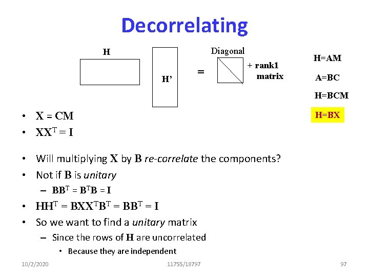
Decorrelating Diagonal H H’ = + rank 1 matrix H=AM A=BC H=BCM • X = CM • XXT = I H=BX • Will multiplying X by B re-correlate the components? • Not if B is unitary – BBT = BTB = I • HHT = BXXTBT = BBT = I • So we want to find a unitary matrix – Since the rows of H are uncorrelated • Because they are independent 10/2/2020 11755/18797 97

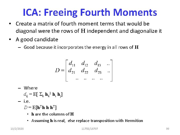
ICA: Freeing Fourth Moments • We have E[xi xj] = 0 if i != j – Already been decorrelated • A=BC, H = BCM, X = CM, H = BX • The fourth moments of H have the form: E[hi hj hk hl] • If the rows of H were independent E[hi hj hk hl] = E[hi] E[hj] E[hk] E[hl] • Solution: Compute B such that the fourth moments of H = BX are decoupled – While ensuring that B is Unitary 10/2/2020 11755/18797 98

ICA: Freeing Fourth Moments • Create a matrix of fourth moment terms that would be diagonal were the rows of H independent and diagonalize it • A good candidate – Good because it incorporates the energy in all rows of H – Where dij = E[ Sk hk 2 hi hj] – i. e. D = E[h. Th h h. T] • h are the columns of H • Assuming h is real, else replace transposition with Hermition 10/2/2020 11755/18797 99

ICA: The D matrix dij = E[ Sk hk 2 hi hj] = Sum of squares of all components Shk 2 jth component hi hj Shk 2 hi hj • Average above term across all columns of H 10/2/2020 11755/18797 100

ICA: The D matrix dij = E[ Sk hk 2 hi hj] = • If the hi terms were independent – For i != j – Centered: E[hj] = 0 E[ Sk hk 2 hi hj]=0 for i != j – For i = j • Thus, if the hi terms were independent, dij = 0 if i != j • i. e. , if hi were independent, D would be a diagonal matrix 10/2/2020 – Let us diagonalize D 11755/18797 101

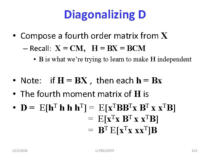
Diagonalizing D • Compose a fourth order matrix from X – Recall: X = CM, H = BX = BCM • B is what we’re trying to learn to make H independent • Note: if H = BX , then each h = Bx • The fourth moment matrix of H is • D = E[h. T h h h. T] = E[x. TBBTx BT x x. TB] = E[x. Tx BT x x. TB] = BT E[x. Tx xx. T]B 10/2/2020 11755/18797 102

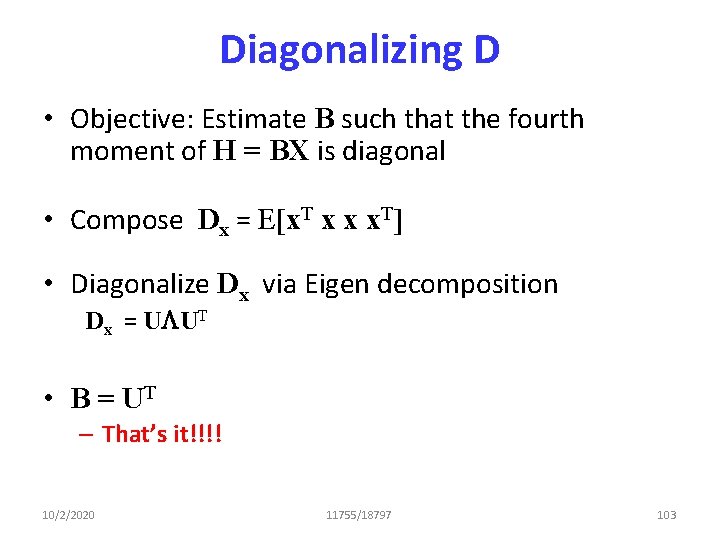
Diagonalizing D • Objective: Estimate B such that the fourth moment of H = BX is diagonal • Compose Dx = E[x. T x x x. T] • Diagonalize Dx via Eigen decomposition Dx = ULUT • B = UT – That’s it!!!! 10/2/2020 11755/18797 103

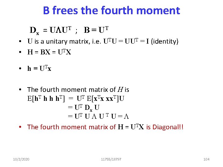
B frees the fourth moment Dx = ULUT ; B = UT • U is a unitary matrix, i. e. UTU = UUT = I (identity) • H = BX = UTX • h = U Tx • The fourth moment matrix of H is E[h. T h h h. T] = UT E[x. Tx xx. T]U = UT Dx U = UT U L U T U = L • The fourth moment matrix of H = UTX is Diagonal!! 10/2/2020 11755/18797 104

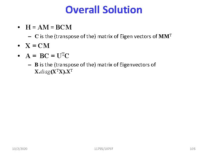
Overall Solution • H = AM = BCM – C is the (transpose of the) matrix of Eigen vectors of MMT • X = CM • A = BC = UTC – B is the (transpose of the) matrix of Eigenvectors of X. diag(XTX). XT 10/2/2020 11755/18797 105

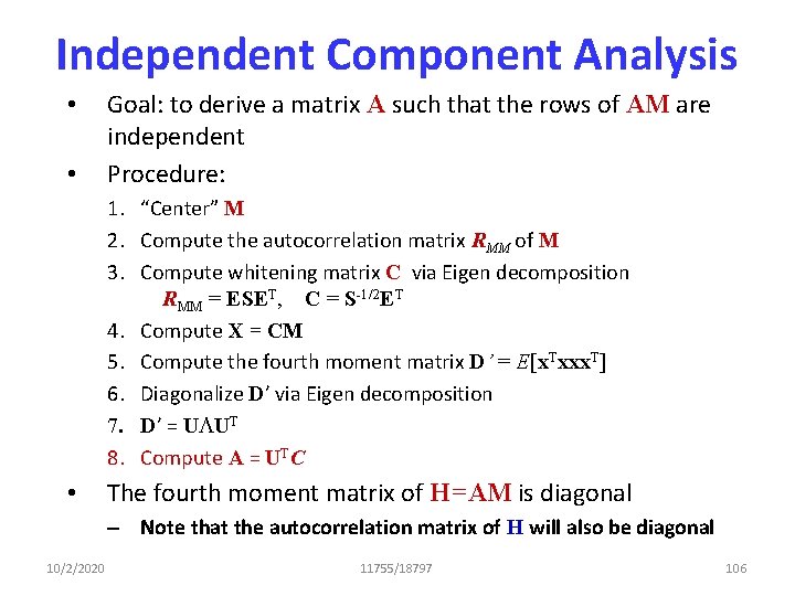
Independent Component Analysis • • Goal: to derive a matrix A such that the rows of AM are independent Procedure: 1. “Center” M 2. Compute the autocorrelation matrix RMM of M 3. Compute whitening matrix C via Eigen decomposition RMM = ESET, C = S-1/2 ET 4. Compute X = CM 5. Compute the fourth moment matrix D’ = E[x. Txxx. T] 6. Diagonalize D’ via Eigen decomposition 7. D’ = ULUT 8. Compute A = UTC • The fourth moment matrix of H=AM is diagonal – Note that the autocorrelation matrix of H will also be diagonal 10/2/2020 11755/18797 106

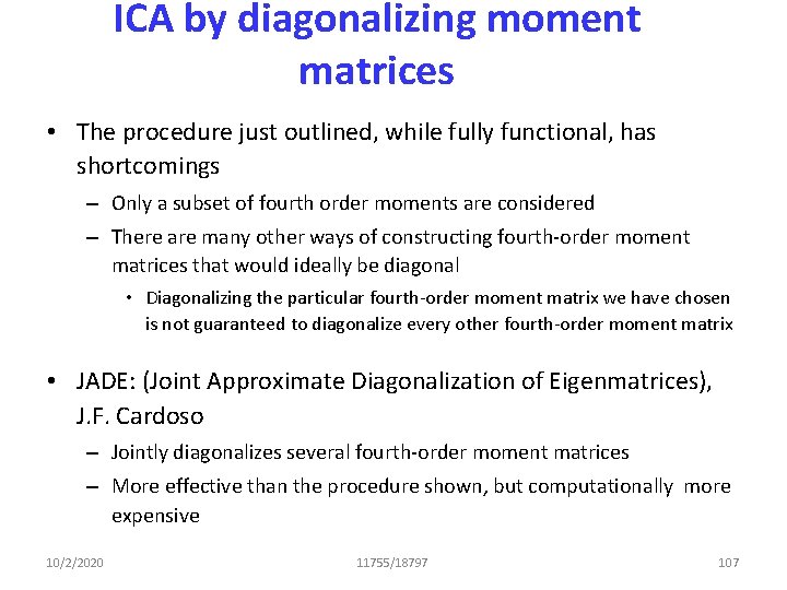
ICA by diagonalizing moment matrices • The procedure just outlined, while fully functional, has shortcomings – Only a subset of fourth order moments are considered – There are many other ways of constructing fourth-order moment matrices that would ideally be diagonal • Diagonalizing the particular fourth-order moment matrix we have chosen is not guaranteed to diagonalize every other fourth-order moment matrix • JADE: (Joint Approximate Diagonalization of Eigenmatrices), J. F. Cardoso – Jointly diagonalizes several fourth-order moment matrices – More effective than the procedure shown, but computationally more expensive 10/2/2020 11755/18797 107

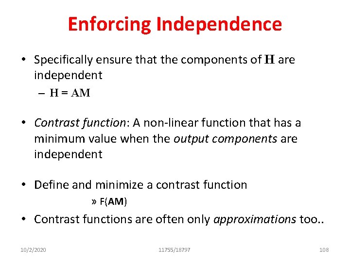
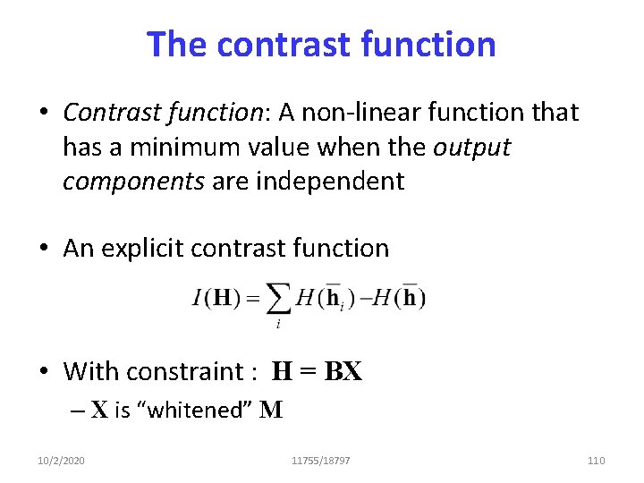
Enforcing Independence • Specifically ensure that the components of H are independent – H = AM • Contrast function: A non-linear function that has a minimum value when the output components are independent • Define and minimize a contrast function » F(AM) • Contrast functions are often only approximations too. . 10/2/2020 11755/18797 108

A note on pre-whitening • The mixed signal is usually “prewhitened” – Normalize variance along all directions – Eliminate second-order dependence • Eigen decomposition MMT = ESET • C = S-1/2 ET • Can use first K columns of E only if only K independent sources are expected – In microphone array setup – only K < M sources • X = CM – E[xixj] = dij for centered signal 10/2/2020 11755/18797 109

The contrast function • Contrast function: A non-linear function that has a minimum value when the output components are independent • An explicit contrast function • With constraint : H = BX – X is “whitened” M 10/2/2020 11755/18797 110

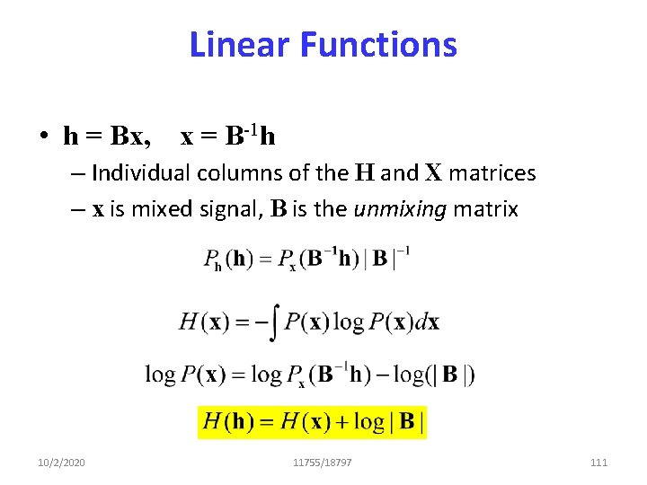
Linear Functions • h = Bx, x = B-1 h – Individual columns of the H and X matrices – x is mixed signal, B is the unmixing matrix 10/2/2020 11755/18797 111

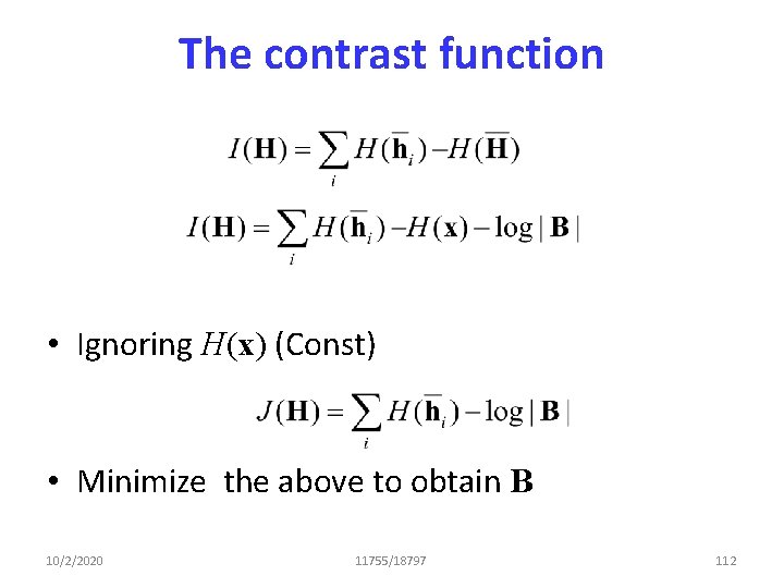
The contrast function • Ignoring H(x) (Const) • Minimize the above to obtain B 10/2/2020 11755/18797 112

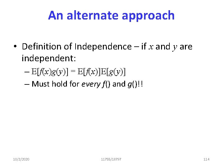
An alternate approach • Definition of Independence – if x and y are independent: – E[f(x)g(y)] = E[f(x)]E[g(y)] – Must hold for every f() and g()!! 10/2/2020 11755/18797 114

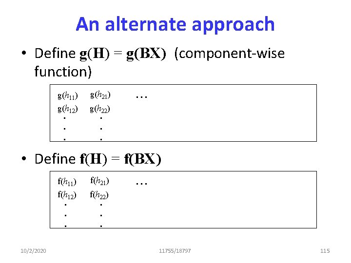
An alternate approach • Define g(H) = g(BX) (component-wise function) g(h 11) g(h 21) g(h 12). . . g(h 22). . . • Define f(H) = f(BX) 10/2/2020 f(h 11) f(h 21) f(h 12). . . f(h 22). . . 11755/18797 115

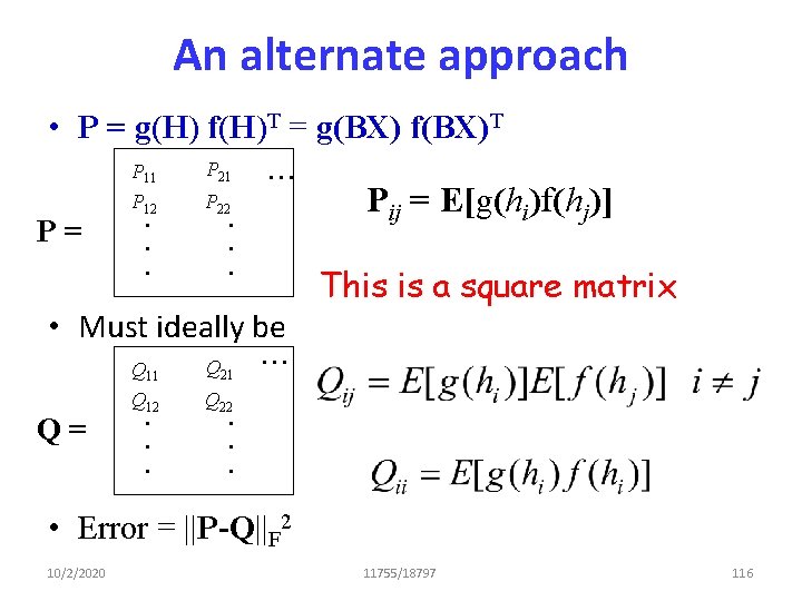
An alternate approach • P = g(H) f(H)T = g(BX) f(BX)T P = P 11 P 21 P 12. . . P 22. . . Q 11 Q 21 Q 12. . . Q 22. . . Pij = E[g(hi)f(hj)] This is a square matrix • Must ideally be Q= . . . • Error = ||P-Q||F 2 10/2/2020 11755/18797 116

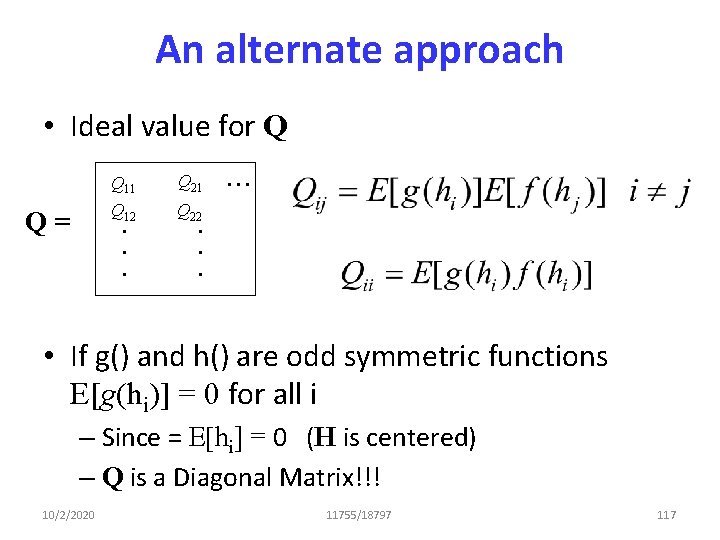
An alternate approach • Ideal value for Q Q= Q 11 Q 21 Q 12. . . Q 22. . . • If g() and h() are odd symmetric functions E[g(hi)] = 0 for all i – Since = E[hi] = 0 (H is centered) – Q is a Diagonal Matrix!!! 10/2/2020 11755/18797 117

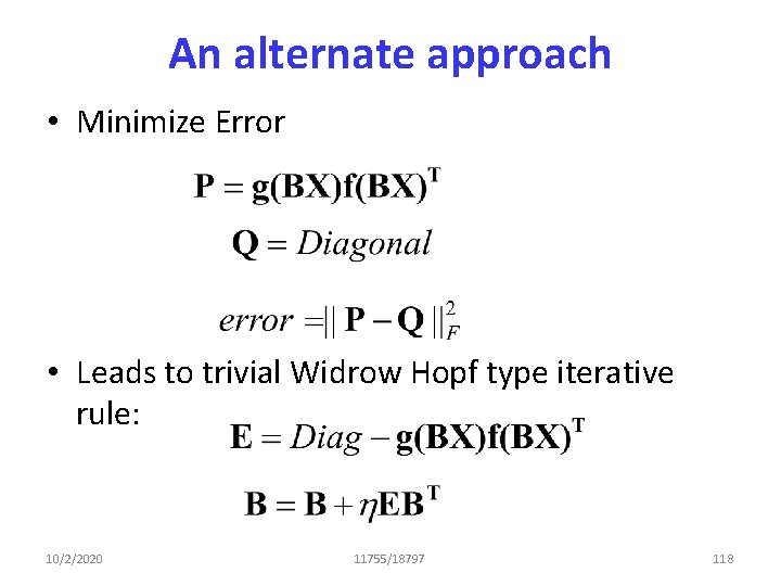
An alternate approach • Minimize Error • Leads to trivial Widrow Hopf type iterative rule: 10/2/2020 11755/18797 118

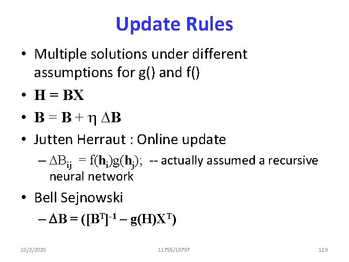
Update Rules • Multiple solutions under different assumptions for g() and f() • H = BX • B = B + h DB • Jutten Herraut : Online update – DBij = f(hi)g(hj); -- actually assumed a recursive neural network • Bell Sejnowski – DB = ([BT]-1 – g(H)XT) 10/2/2020 11755/18797 119

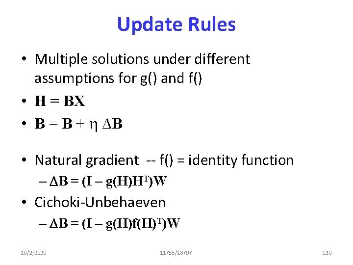
Update Rules • Multiple solutions under different assumptions for g() and f() • H = BX • B = B + h DB • Natural gradient -- f() = identity function – DB = (I – g(H)HT)W • Cichoki-Unbehaeven – DB = (I – g(H)f(H)T)W 10/2/2020 11755/18797 120

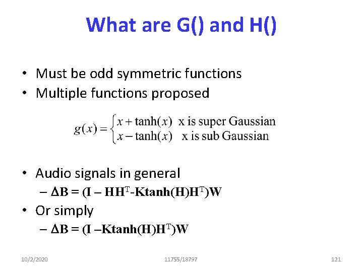
What are G() and H() • Must be odd symmetric functions • Multiple functions proposed • Audio signals in general – DB = (I – HHT-Ktanh(H)HT)W • Or simply – DB = (I –Ktanh(H)HT)W 10/2/2020 11755/18797 121

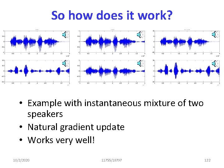
So how does it work? • Example with instantaneous mixture of two speakers • Natural gradient update • Works very well! 10/2/2020 11755/18797 122

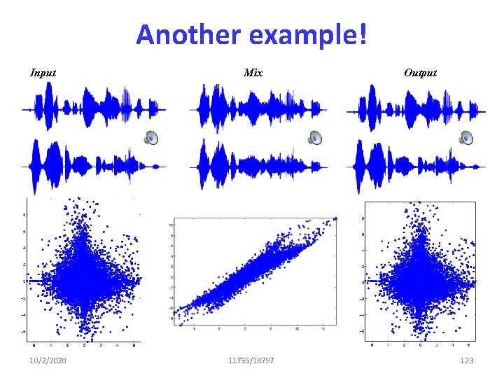
Another example! Input 10/2/2020 Mix 11755/18797 Output 123

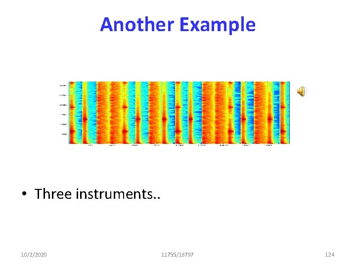
Another Example • Three instruments. . 10/2/2020 11755/18797 124

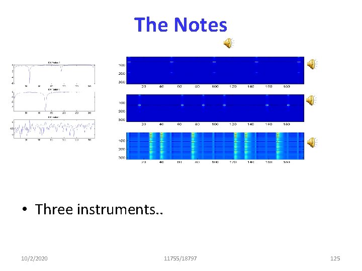
The Notes • Three instruments. . 10/2/2020 11755/18797 125

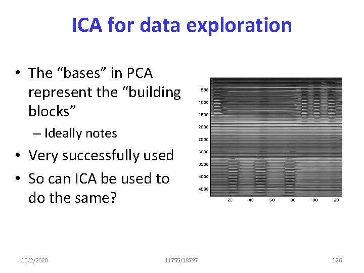
ICA for data exploration • The “bases” in PCA represent the “building blocks” – Ideally notes • Very successfully used • So can ICA be used to do the same? 10/2/2020 11755/18797 126

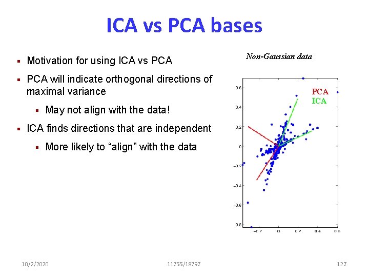
ICA vs PCA bases § Motivation for using ICA vs PCA § PCA will indicate orthogonal directions of maximal variance § § May not align with the data! Non-Gaussian data PCA ICA finds directions that are independent § More likely to “align” with the data 10/2/2020 11755/18797 127

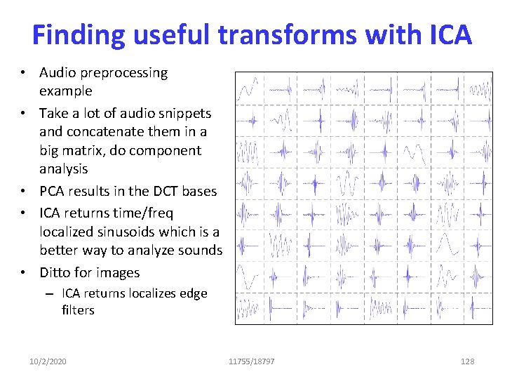
Finding useful transforms with ICA • Audio preprocessing example • Take a lot of audio snippets and concatenate them in a big matrix, do component analysis • PCA results in the DCT bases • ICA returns time/freq localized sinusoids which is a better way to analyze sounds • Ditto for images – ICA returns localizes edge filters 10/2/2020 11755/18797 128

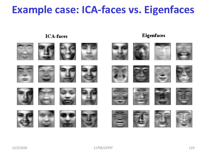
Example case: ICA-faces vs. Eigenfaces ICA-faces 10/2/2020 11755/18797 129

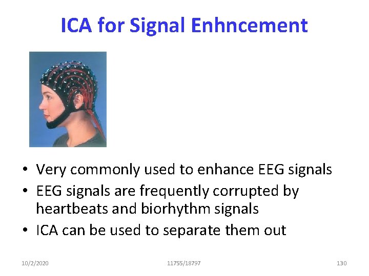
ICA for Signal Enhncement • Very commonly used to enhance EEG signals • EEG signals are frequently corrupted by heartbeats and biorhythm signals • ICA can be used to separate them out 10/2/2020 11755/18797 130

So how does that work? • There are 12 notes in the segment, hence we try to estimate 12 notes. . 10/2/2020 11755/18797 131

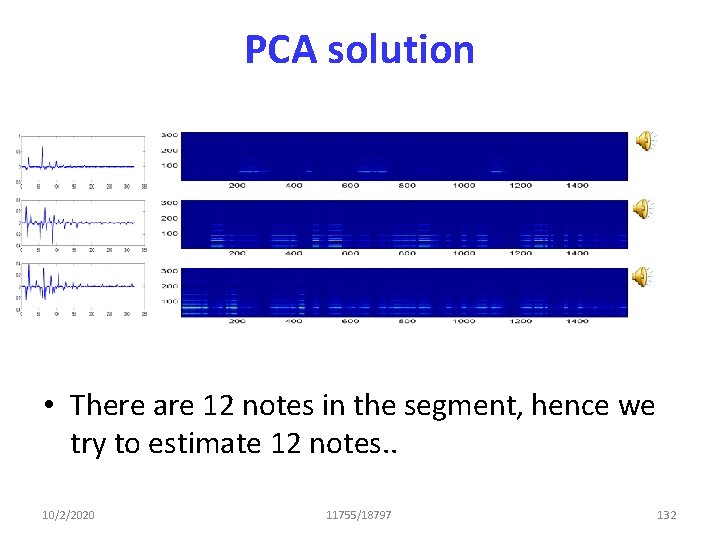
PCA solution • There are 12 notes in the segment, hence we try to estimate 12 notes. . 10/2/2020 11755/18797 132

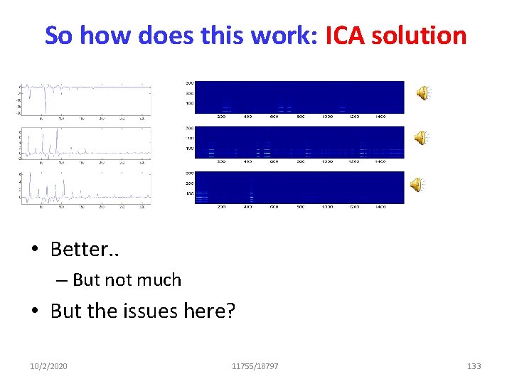
So how does this work: ICA solution • Better. . – But not much • But the issues here? 10/2/2020 11755/18797 133

ICA Issues • No sense of order – Unlike PCA • Get K independent directions, but does not have a notion of the “best” direction – So the sources can come in any order – Permutation invariance • Does not have sense of scaling – Scaling the signal does not affect independence • Outputs are scaled versions of desired signals in permuted order – In the best case – In worse case, output are not desired signals at all. . 10/2/2020 11755/18797 134

What else went wrong? • Notes are not independent – Only one note plays at a time – If one note plays, other notes are not playing • Will deal with these later in the course. . 10/2/2020 11755/18797 135