Machine Learning for Signal Processing Fundamentals of Linear

Machine Learning for Signal Processing Fundamentals of Linear Algebra Class 2. 2 Sep 2014 Instructor: Bhiksha Raj 2 Sep 2014 11 -755/18 -797 1

Administrivia • Info on second TA still awaited from ECE • Registration: Anyone on waitlist still? • Homework 1: Will appear on Thursday. – Linear algebra 2 Sep 2014 11 -755/18 -797 2

Overview • • • Vectors and matrices Basic vector/matrix operations Vector products Matrix products Various matrix types Projections 2 Sep 2014 11 -755/18 -797 3

Book • Fundamentals of Linear Algebra, Gilbert Strang • Important to be very comfortable with linear algebra – Appears repeatedly in the form of Eigen analysis, SVD, Factor analysis – Appears through various properties of matrices that are used in machine learning – Often used in the processing of data of various kinds – Will use sound and images as examples • Today’s lecture: Definitions – Very small subset of all that’s used – Important subset, intended to help you recollect 2 Sep 2014 11 -755/18 -797 4

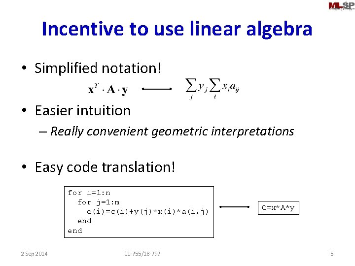
Incentive to use linear algebra • Simplified notation! • Easier intuition – Really convenient geometric interpretations • Easy code translation! for i=1: n for j=1: m c(i)=c(i)+y(j)*x(i)*a(i, j) end 2 Sep 2014 11 -755/18 -797 C=x*A*y 5

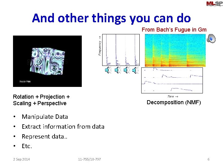
And other things you can do Frequency From Bach’s Fugue in Gm Rotation + Projection + Scaling + Perspective • • Time Decomposition (NMF) Manipulate Data Extract information from data Represent data. . Etc. 2 Sep 2014 11 -755/18 -797 6

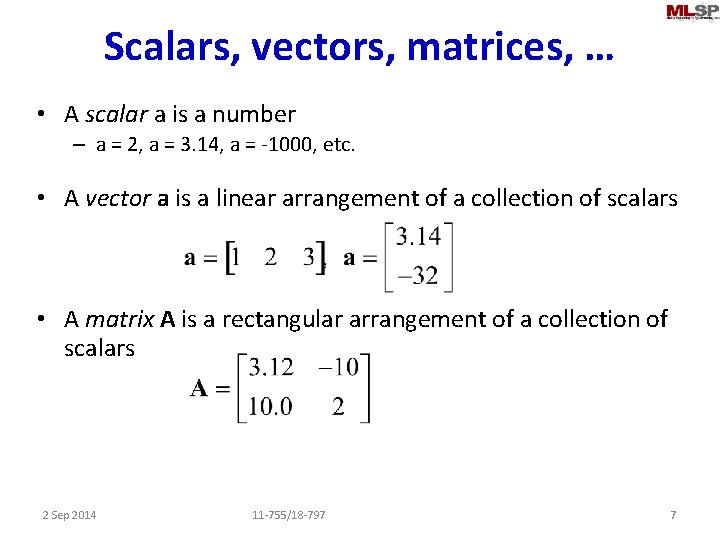
Scalars, vectors, matrices, … • A scalar a is a number – a = 2, a = 3. 14, a = -1000, etc. • A vector a is a linear arrangement of a collection of scalars • A matrix A is a rectangular arrangement of a collection of scalars 2 Sep 2014 11 -755/18 -797 7

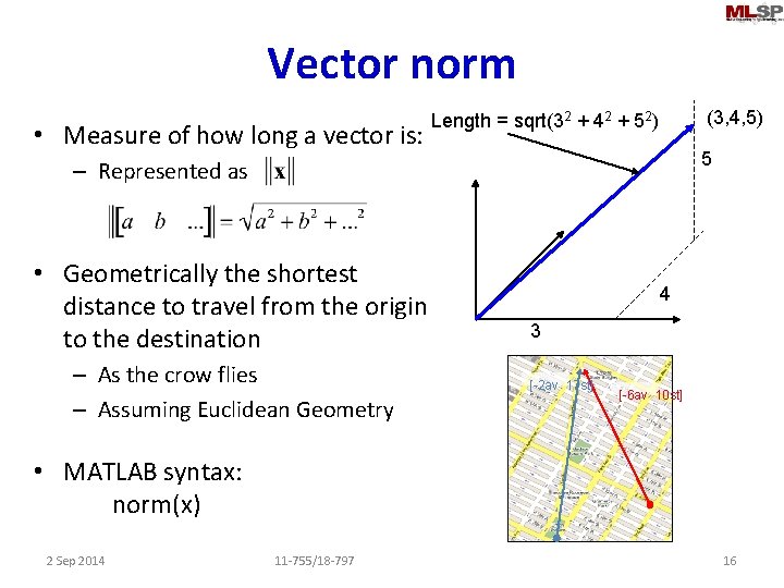
Vectors in the abstract • Ordered collection of numbers – Examples: [3 4 5], [a b c d], . . – [3 4 5] != [4 3 5] Order is important • Typically viewed as identifying (the path from origin to) a location in an N-dimensional space (3, 4, 5) 5 (4, 3, 5) 3 z y 4 x 2 Sep 2014 11 -755/18 -797 8

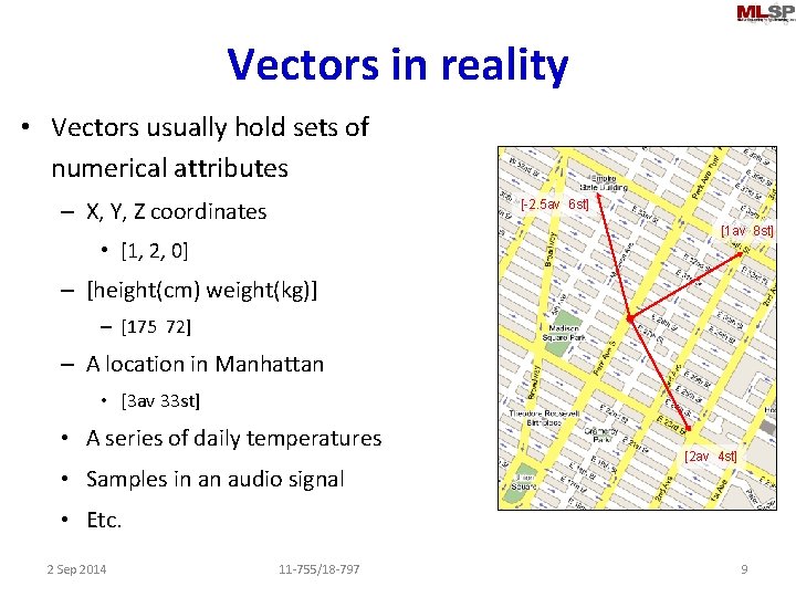
Vectors in reality • Vectors usually hold sets of numerical attributes – X, Y, Z coordinates [-2. 5 av 6 st] [1 av 8 st] • [1, 2, 0] – [height(cm) weight(kg)] – [175 72] – A location in Manhattan • [3 av 33 st] • A series of daily temperatures • Samples in an audio signal [2 av 4 st] • Etc. 2 Sep 2014 11 -755/18 -797 9

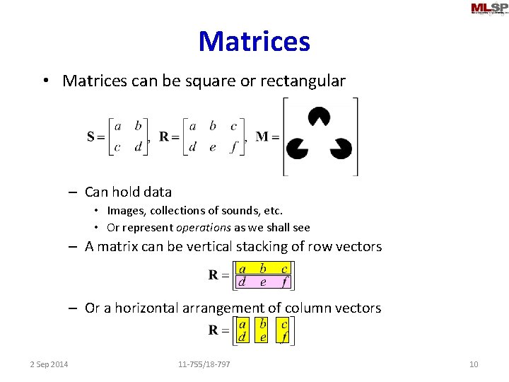
Matrices • Matrices can be square or rectangular – Can hold data • Images, collections of sounds, etc. • Or represent operations as we shall see – A matrix can be vertical stacking of row vectors – Or a horizontal arrangement of column vectors 2 Sep 2014 11 -755/18 -797 10

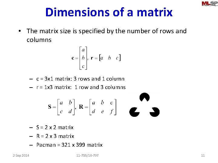
Dimensions of a matrix • The matrix size is specified by the number of rows and columns – c = 3 x 1 matrix: 3 rows and 1 column – r = 1 x 3 matrix: 1 row and 3 columns – S = 2 x 2 matrix – R = 2 x 3 matrix – Pacman = 321 x 399 matrix 2 Sep 2014 11 -755/18 -797 11

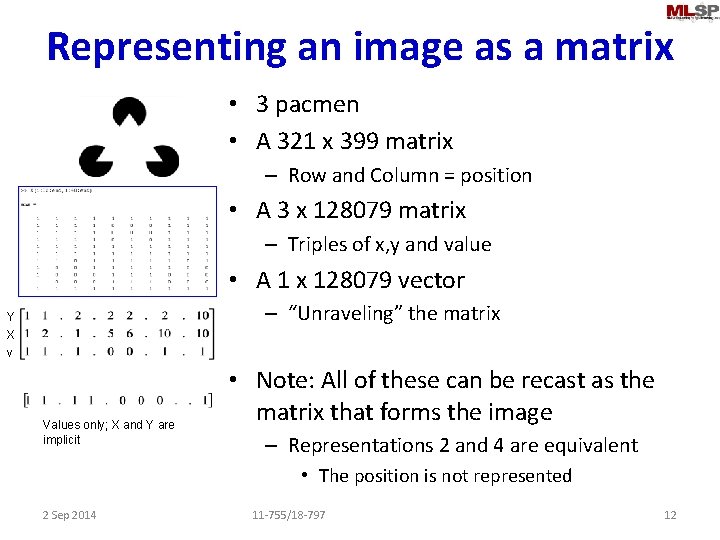
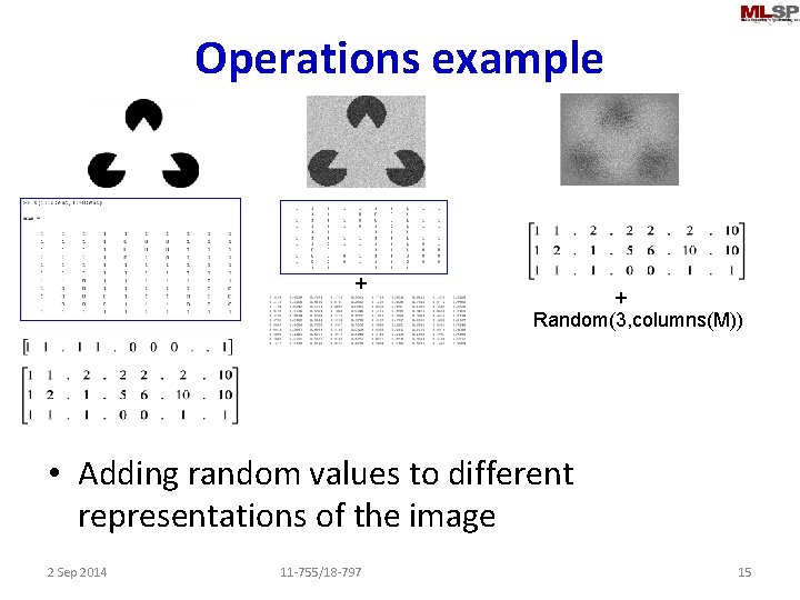
Representing an image as a matrix • 3 pacmen • A 321 x 399 matrix – Row and Column = position • A 3 x 128079 matrix – Triples of x, y and value • A 1 x 128079 vector – “Unraveling” the matrix Y X v Values only; X and Y are implicit • Note: All of these can be recast as the matrix that forms the image – Representations 2 and 4 are equivalent • The position is not represented 2 Sep 2014 11 -755/18 -797 12

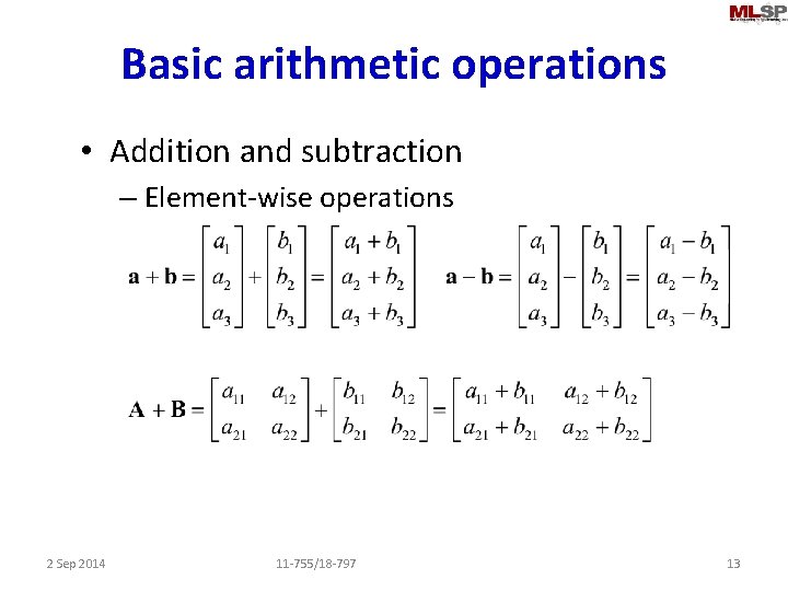
Basic arithmetic operations • Addition and subtraction – Element-wise operations 2 Sep 2014 11 -755/18 -797 13

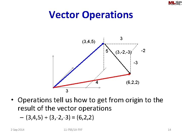
Vector Operations 3 (3, 4, 5) 5 -2 (3, -2, -3) -3 4 (6, 2, 2) 3 • Operations tell us how to get from origin to the result of the vector operations – (3, 4, 5) + (3, -2, -3) = (6, 2, 2) 2 Sep 2014 11 -755/18 -797 14

Operations example + + Random(3, columns(M)) • Adding random values to different representations of the image 2 Sep 2014 11 -755/18 -797 15

Vector norm • Measure of how long a vector is: (3, 4, 5) Length = sqrt(32 + 42 + 52) 5 – Represented as • Geometrically the shortest distance to travel from the origin to the destination – As the crow flies – Assuming Euclidean Geometry 4 3 [-2 av 17 st] [-6 av 10 st] • MATLAB syntax: norm(x) 2 Sep 2014 11 -755/18 -797 16

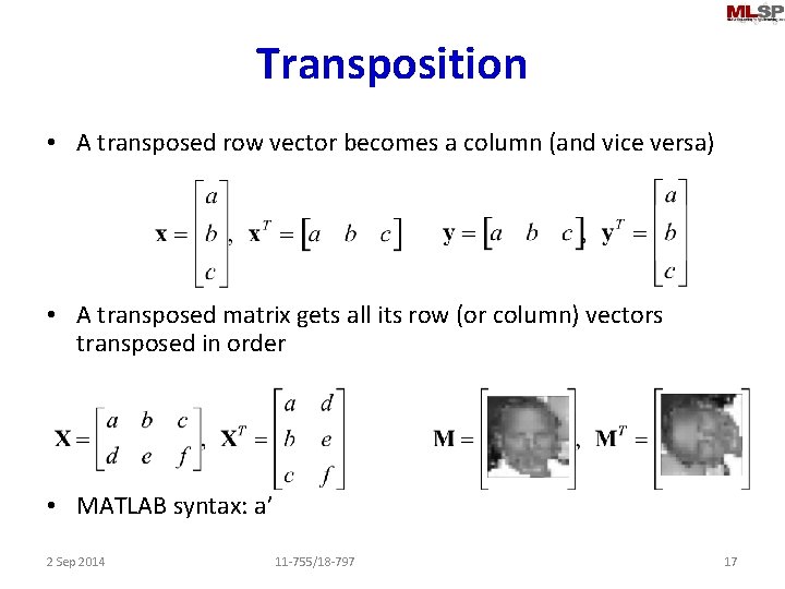
Transposition • A transposed row vector becomes a column (and vice versa) • A transposed matrix gets all its row (or column) vectors transposed in order • MATLAB syntax: a’ 2 Sep 2014 11 -755/18 -797 17

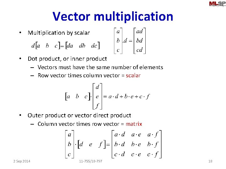
Vector multiplication • Multiplication by scalar • Dot product, or inner product – Vectors must have the same number of elements – Row vector times column vector = scalar • Outer product or vector direct product – Column vector times row vector = matrix 2 Sep 2014 11 -755/18 -797 18

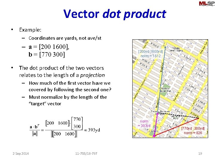
Vector dot product • Example: – Coordinates are yards, not ave/st – a = [200 1600], b = [770 300] [200 yd 1600 yd] norm ≈ 1612 • The dot product of the two vectors relates to the length of a projection – How much of the first vector have we covered by following the second one? – Must normalize by the length of the “target” vector norm ≈ 393 yd 2 Sep 2014 11 -755/18 -797 [770 yd 300 yd] norm ≈ 826 19

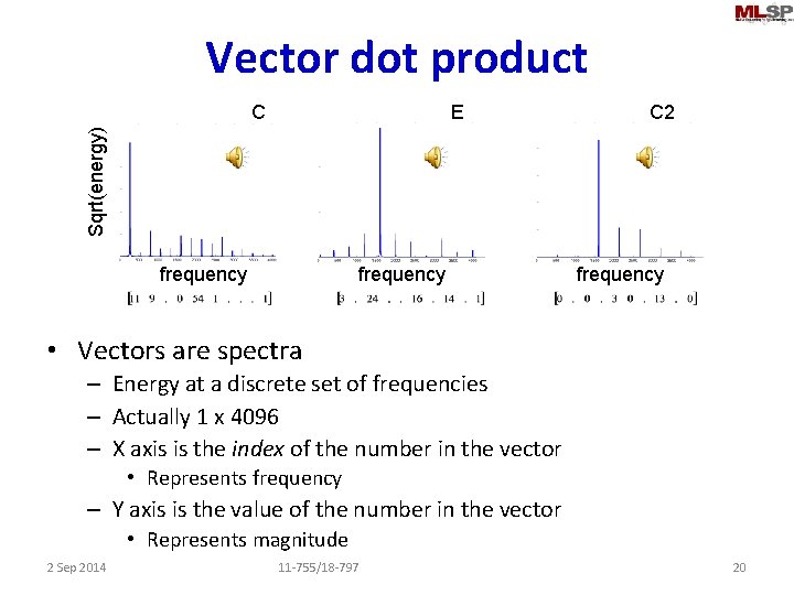
Vector dot product E C 2 Sqrt(energy) C frequency • Vectors are spectra – Energy at a discrete set of frequencies – Actually 1 x 4096 – X axis is the index of the number in the vector • Represents frequency – Y axis is the value of the number in the vector • Represents magnitude 2 Sep 2014 11 -755/18 -797 20

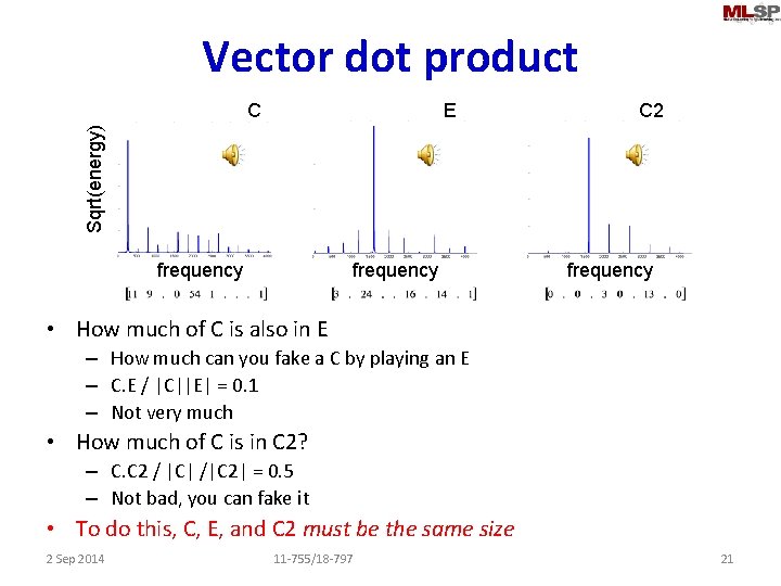
Vector dot product E C 2 Sqrt(energy) C frequency • How much of C is also in E – How much can you fake a C by playing an E – C. E / |C||E| = 0. 1 – Not very much • How much of C is in C 2? – C. C 2 / |C| /|C 2| = 0. 5 – Not bad, you can fake it • To do this, C, E, and C 2 must be the same size 2 Sep 2014 11 -755/18 -797 21

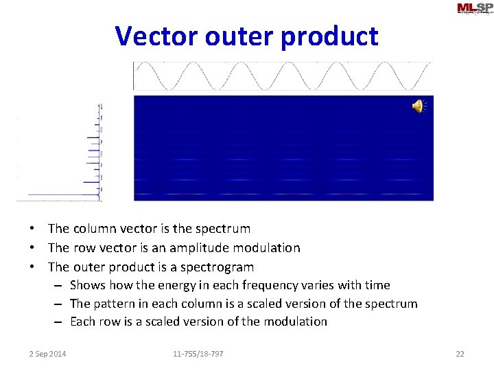
Vector outer product • The column vector is the spectrum • The row vector is an amplitude modulation • The outer product is a spectrogram – Shows how the energy in each frequency varies with time – The pattern in each column is a scaled version of the spectrum – Each row is a scaled version of the modulation 2 Sep 2014 11 -755/18 -797 22

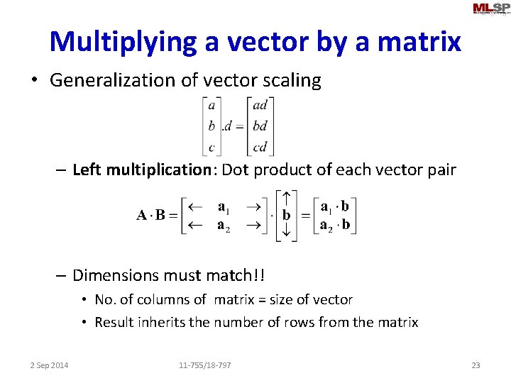
Multiplying a vector by a matrix • Generalization of vector scaling – Left multiplication: Dot product of each vector pair – Dimensions must match!! • No. of columns of matrix = size of vector • Result inherits the number of rows from the matrix 2 Sep 2014 11 -755/18 -797 23

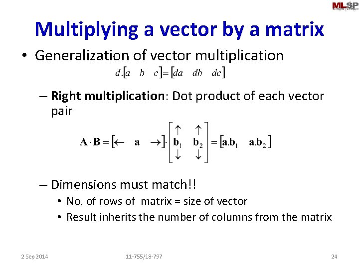
Multiplying a vector by a matrix • Generalization of vector multiplication – Right multiplication: Dot product of each vector pair – Dimensions must match!! • No. of rows of matrix = size of vector • Result inherits the number of columns from the matrix 2 Sep 2014 11 -755/18 -797 24

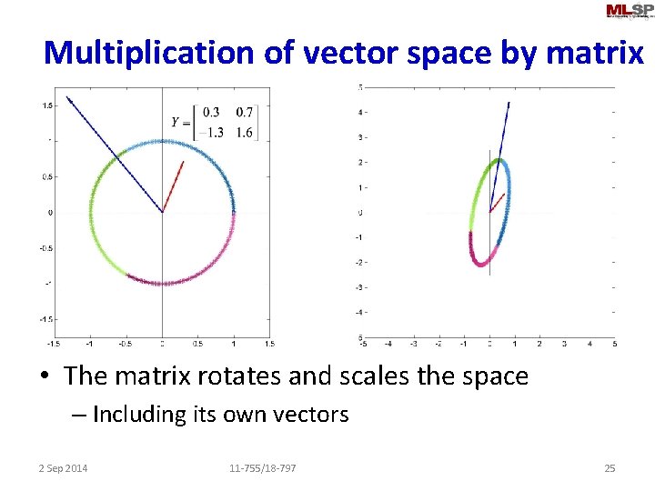
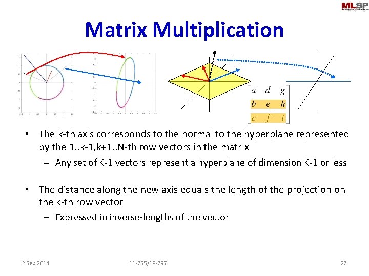
Multiplication of vector space by matrix • The matrix rotates and scales the space – Including its own vectors 2 Sep 2014 11 -755/18 -797 25

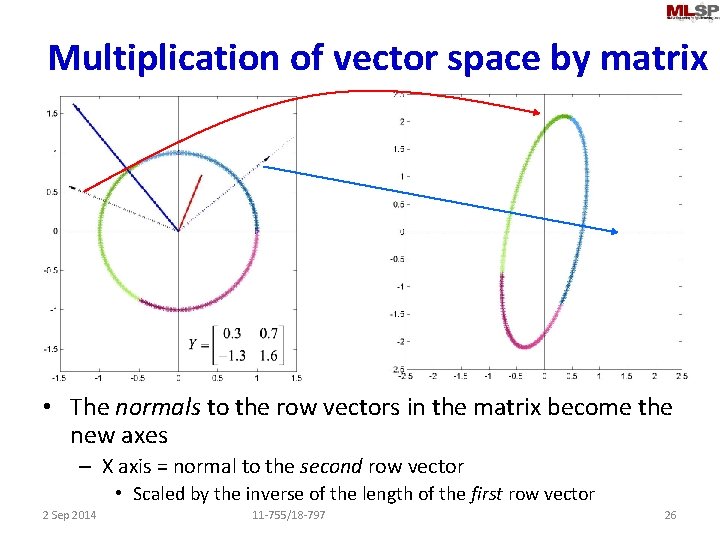
Multiplication of vector space by matrix • The normals to the row vectors in the matrix become the new axes – X axis = normal to the second row vector • Scaled by the inverse of the length of the first row vector 2 Sep 2014 11 -755/18 -797 26

Matrix Multiplication • The k-th axis corresponds to the normal to the hyperplane represented by the 1. . k-1, k+1. . N-th row vectors in the matrix – Any set of K-1 vectors represent a hyperplane of dimension K-1 or less • The distance along the new axis equals the length of the projection on the k-th row vector – Expressed in inverse-lengths of the vector 2 Sep 2014 11 -755/18 -797 27

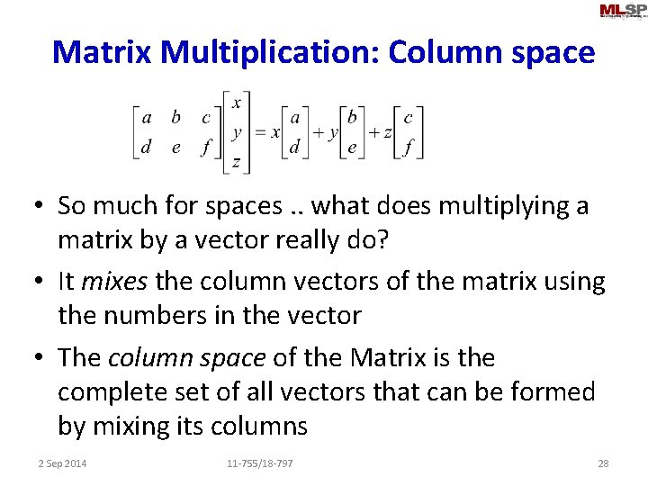
Matrix Multiplication: Column space • So much for spaces. . what does multiplying a matrix by a vector really do? • It mixes the column vectors of the matrix using the numbers in the vector • The column space of the Matrix is the complete set of all vectors that can be formed by mixing its columns 2 Sep 2014 11 -755/18 -797 28

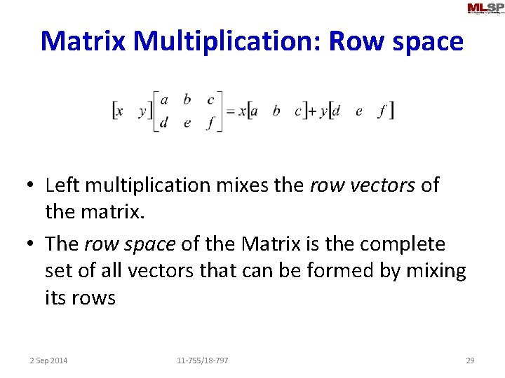
Matrix Multiplication: Row space • Left multiplication mixes the row vectors of the matrix. • The row space of the Matrix is the complete set of all vectors that can be formed by mixing its rows 2 Sep 2014 11 -755/18 -797 29

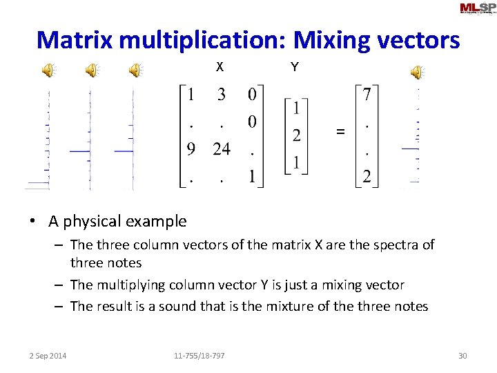
Matrix multiplication: Mixing vectors X Y = • A physical example – The three column vectors of the matrix X are the spectra of three notes – The multiplying column vector Y is just a mixing vector – The result is a sound that is the mixture of the three notes 2 Sep 2014 11 -755/18 -797 30

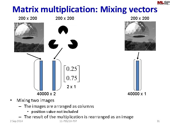
Matrix multiplication: Mixing vectors 200 x 200 2 x 1 40000 x 2 40000 x 1 • Mixing two images – The images are arranged as columns • position value not included – The result of the multiplication is rearranged as an image 2 Sep 2014 11 -755/18 -797 31

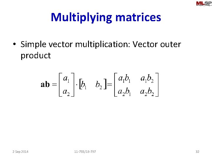
Multiplying matrices • Simple vector multiplication: Vector outer product 2 Sep 2014 11 -755/18 -797 32

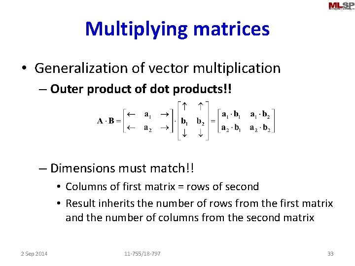
Multiplying matrices • Generalization of vector multiplication – Outer product of dot products!! – Dimensions must match!! • Columns of first matrix = rows of second • Result inherits the number of rows from the first matrix and the number of columns from the second matrix 2 Sep 2014 11 -755/18 -797 33

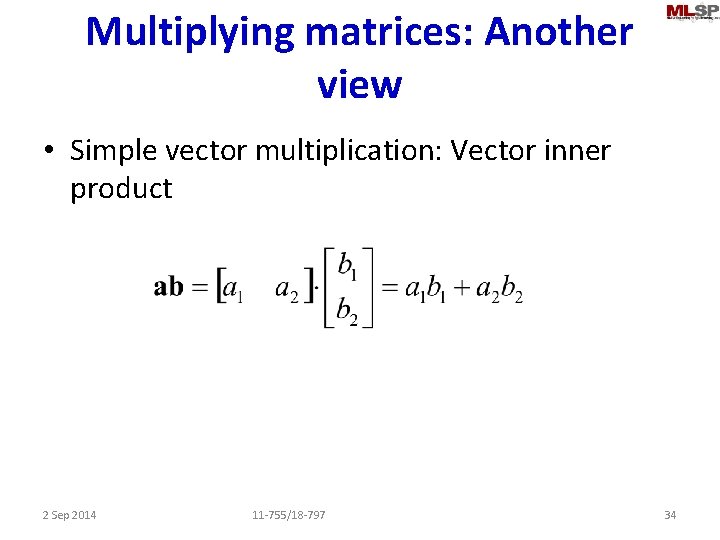
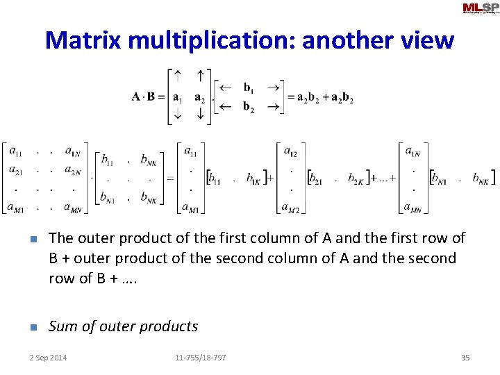
Multiplying matrices: Another view • Simple vector multiplication: Vector inner product 2 Sep 2014 11 -755/18 -797 34

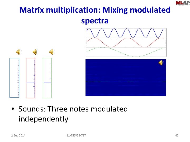
Matrix multiplication: another view n n The outer product of the first column of A and the first row of B + outer product of the second column of A and the second row of B + …. Sum of outer products 2 Sep 2014 11 -755/18 -797 35

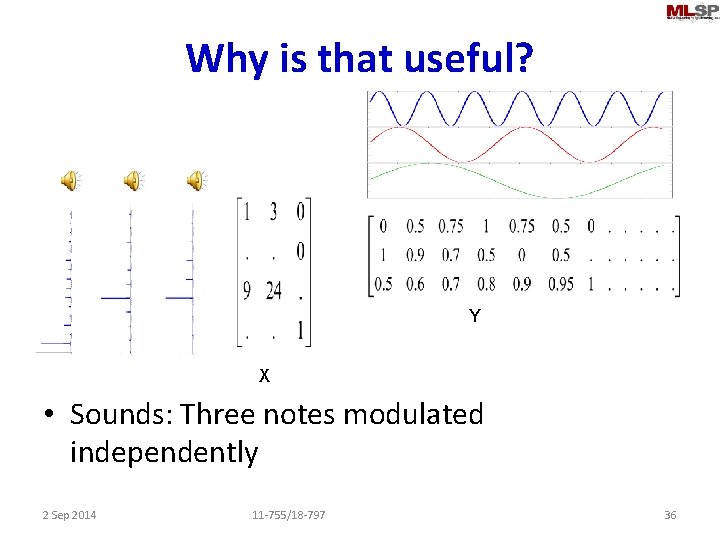
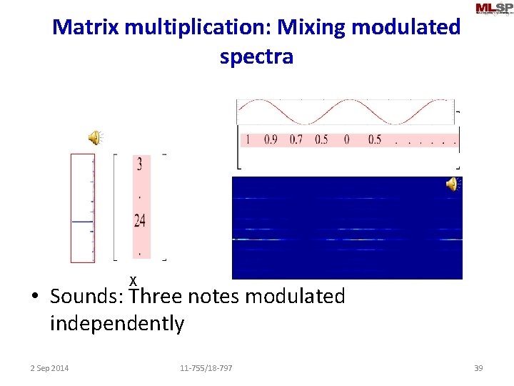
Why is that useful? Y X • Sounds: Three notes modulated independently 2 Sep 2014 11 -755/18 -797 36

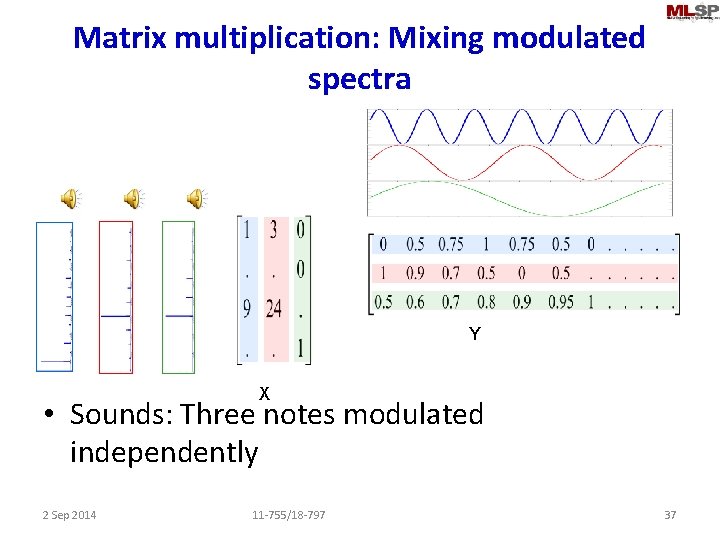
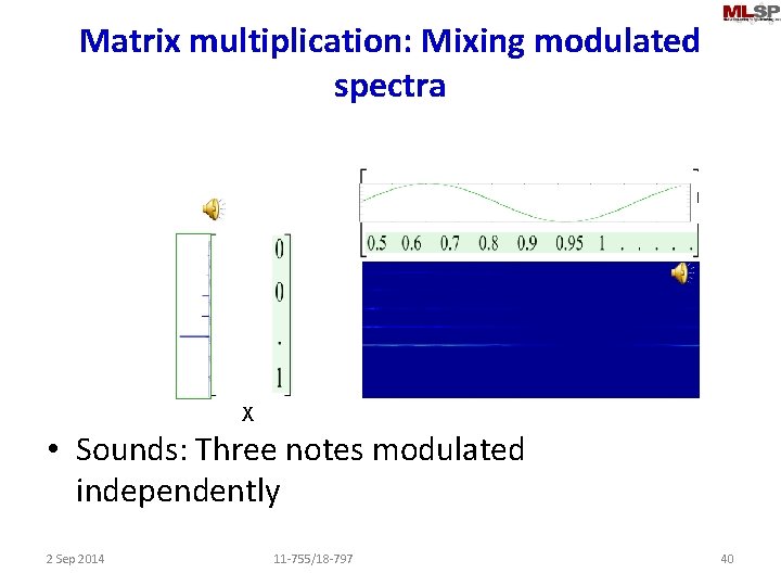
Matrix multiplication: Mixing modulated spectra Y X • Sounds: Three notes modulated independently 2 Sep 2014 11 -755/18 -797 37

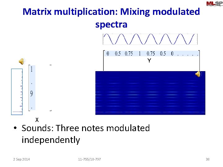
Matrix multiplication: Mixing modulated spectra Y X • Sounds: Three notes modulated independently 2 Sep 2014 11 -755/18 -797 38

Matrix multiplication: Mixing modulated spectra X • Sounds: Three notes modulated independently 2 Sep 2014 11 -755/18 -797 39

Matrix multiplication: Mixing modulated spectra X • Sounds: Three notes modulated independently 2 Sep 2014 11 -755/18 -797 40

Matrix multiplication: Mixing modulated spectra • Sounds: Three notes modulated independently 2 Sep 2014 11 -755/18 -797 41

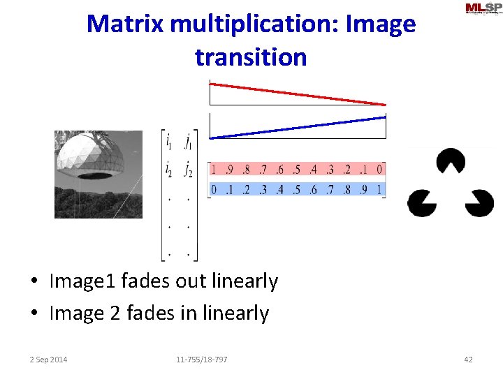
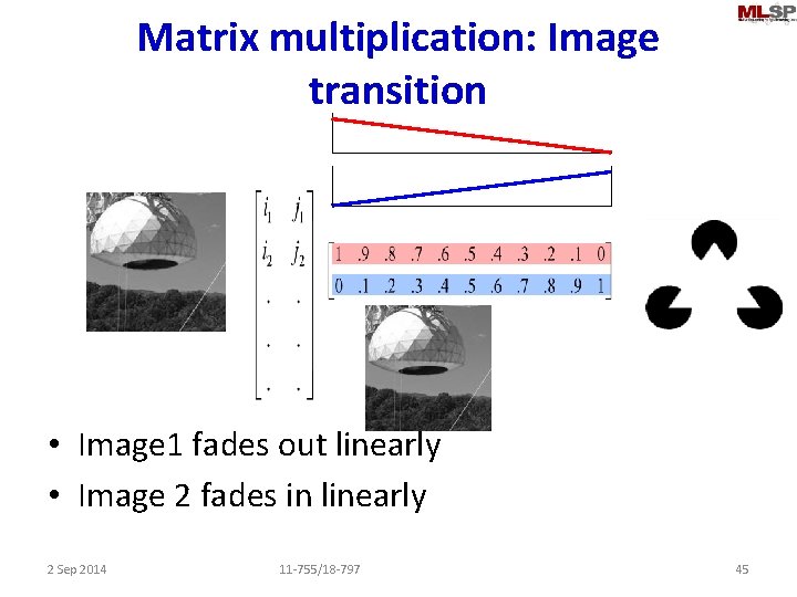
Matrix multiplication: Image transition • Image 1 fades out linearly • Image 2 fades in linearly 2 Sep 2014 11 -755/18 -797 42

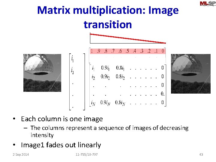
Matrix multiplication: Image transition • Each column is one image – The columns represent a sequence of images of decreasing intensity • Image 1 fades out linearly 2 Sep 2014 11 -755/18 -797 43

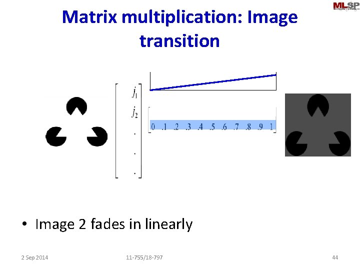
Matrix multiplication: Image transition • Image 2 fades in linearly 2 Sep 2014 11 -755/18 -797 44

Matrix multiplication: Image transition • Image 1 fades out linearly • Image 2 fades in linearly 2 Sep 2014 11 -755/18 -797 45

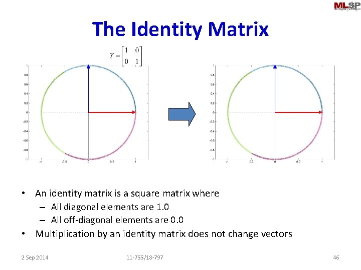
The Identity Matrix • An identity matrix is a square matrix where – All diagonal elements are 1. 0 – All off-diagonal elements are 0. 0 • Multiplication by an identity matrix does not change vectors 2 Sep 2014 11 -755/18 -797 46

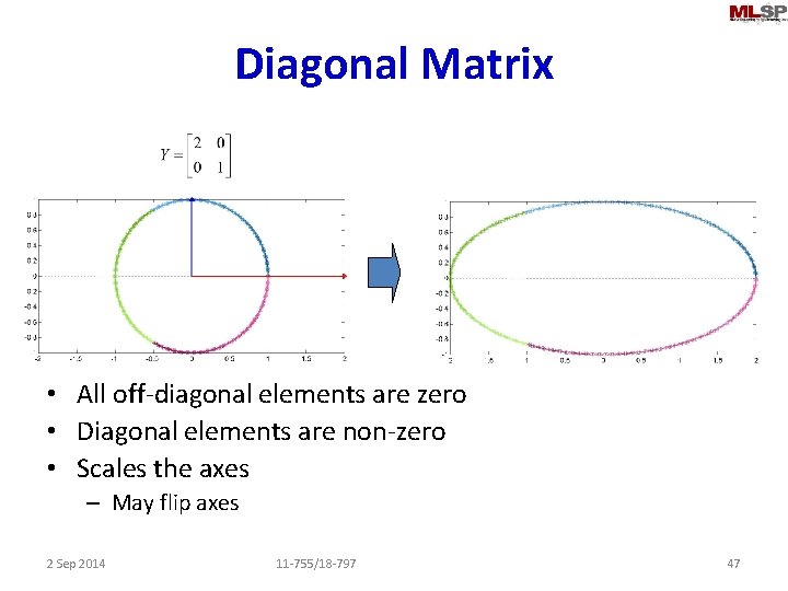
Diagonal Matrix • All off-diagonal elements are zero • Diagonal elements are non-zero • Scales the axes – May flip axes 2 Sep 2014 11 -755/18 -797 47

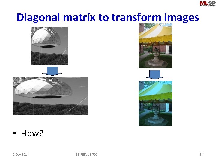
Diagonal matrix to transform images • How? 2 Sep 2014 11 -755/18 -797 48

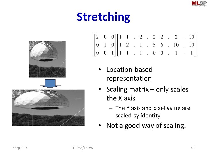
Stretching • Location-based representation • Scaling matrix – only scales the X axis – The Y axis and pixel value are scaled by identity • Not a good way of scaling. 2 Sep 2014 11 -755/18 -797 49

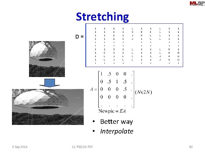
Stretching D= • Better way • Interpolate 2 Sep 2014 11 -755/18 -797 50

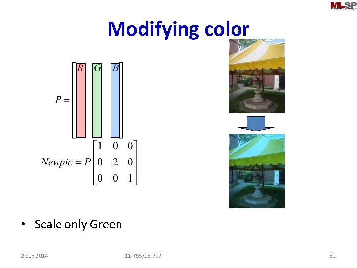
Modifying color • Scale only Green 2 Sep 2014 11 -755/18 -797 51

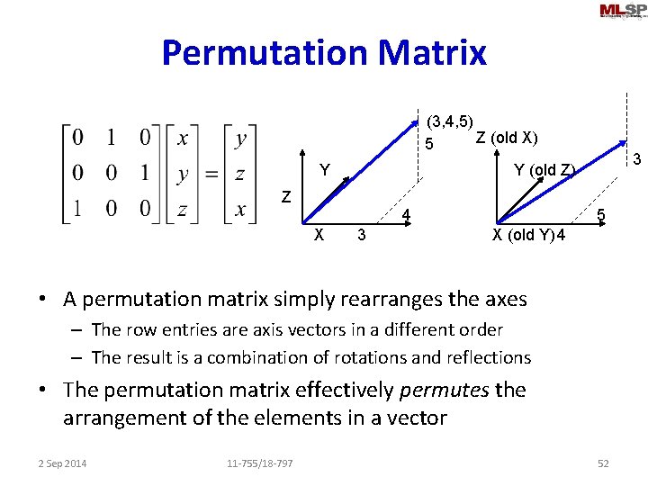
Permutation Matrix (3, 4, 5) Z (old X) 5 Y Z 4 X 3 Y (old Z) 3 5 X (old Y) 4 • A permutation matrix simply rearranges the axes – The row entries are axis vectors in a different order – The result is a combination of rotations and reflections • The permutation matrix effectively permutes the arrangement of the elements in a vector 2 Sep 2014 11 -755/18 -797 52

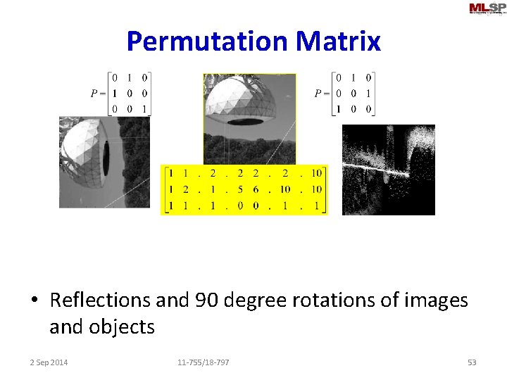
Permutation Matrix • Reflections and 90 degree rotations of images and objects 2 Sep 2014 11 -755/18 -797 53

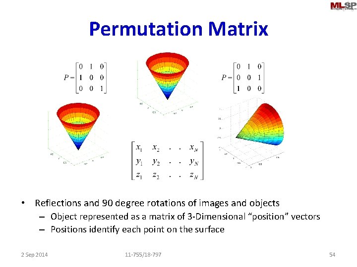
Permutation Matrix • Reflections and 90 degree rotations of images and objects – Object represented as a matrix of 3 -Dimensional “position” vectors – Positions identify each point on the surface 2 Sep 2014 11 -755/18 -797 54

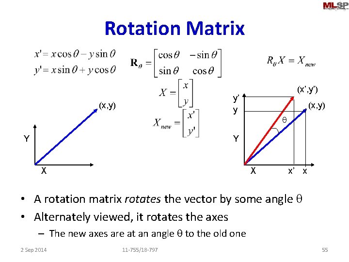
Rotation Matrix (x’, y’) y’ y (x, y) Y (x, y) q Y X X x’ x • A rotation matrix rotates the vector by some angle q • Alternately viewed, it rotates the axes – The new axes are at an angle q to the old one 2 Sep 2014 11 -755/18 -797 55

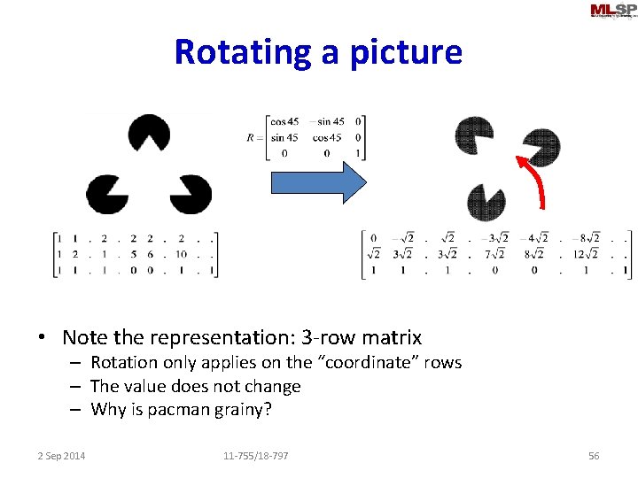
Rotating a picture • Note the representation: 3 -row matrix – Rotation only applies on the “coordinate” rows – The value does not change – Why is pacman grainy? 2 Sep 2014 11 -755/18 -797 56

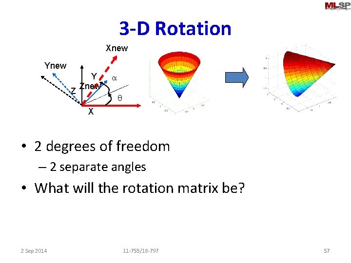
3 -D Rotation Xnew Ynew Z Y Znew a q X • 2 degrees of freedom – 2 separate angles • What will the rotation matrix be? 2 Sep 2014 11 -755/18 -797 57

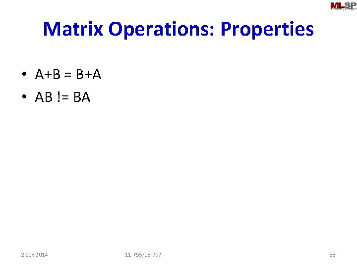
Matrix Operations: Properties • A+B = B+A • AB != BA 2 Sep 2014 11 -755/18 -797 58

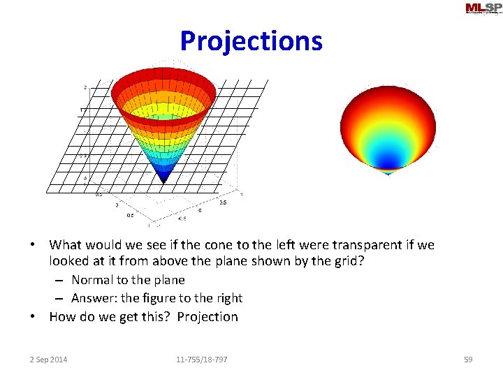
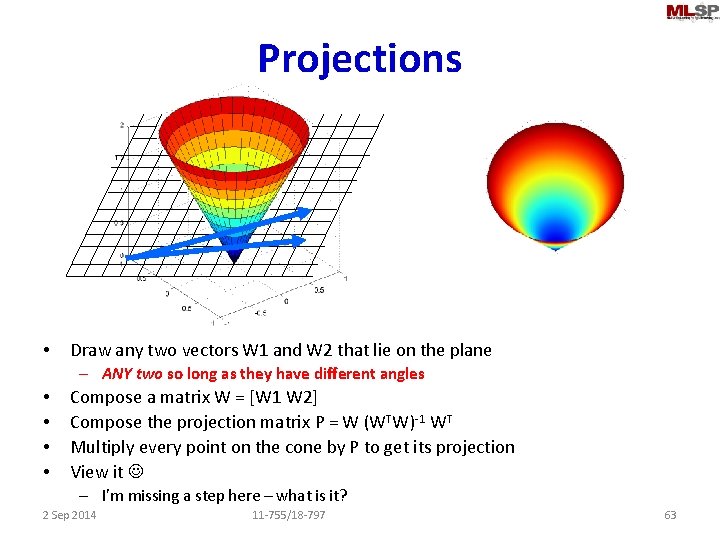
Projections • What would we see if the cone to the left were transparent if we looked at it from above the plane shown by the grid? – Normal to the plane – Answer: the figure to the right • How do we get this? Projection 2 Sep 2014 11 -755/18 -797 59

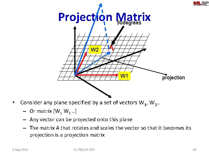
Projection Matrix 90 degrees W 2 W 1 projection • Consider any plane specified by a set of vectors W 1, W 2. . – Or matrix [W 1 W 2. . ] – Any vector can be projected onto this plane – The matrix A that rotates and scales the vector so that it becomes its projection is a projection matrix 2 Sep 2014 11 -755/18 -797 60

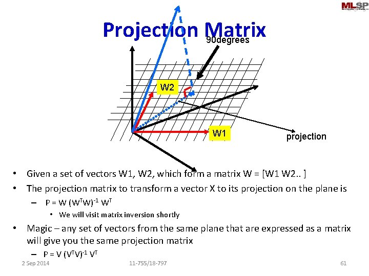
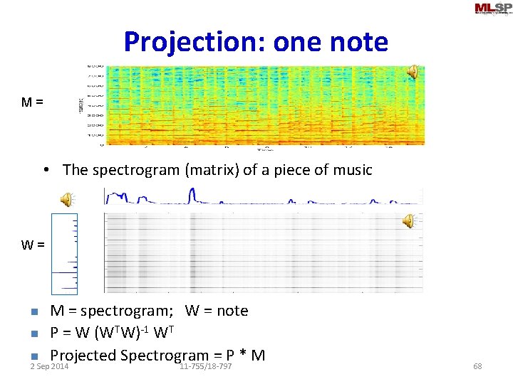
Projection Matrix 90 degrees W 2 W 1 projection • Given a set of vectors W 1, W 2, which form a matrix W = [W 1 W 2. . ] • The projection matrix to transform a vector X to its projection on the plane is – P = W (WTW)-1 WT • We will visit matrix inversion shortly • Magic – any set of vectors from the same plane that are expressed as a matrix will give you the same projection matrix – P = V (VTV)-1 VT 2 Sep 2014 11 -755/18 -797 61

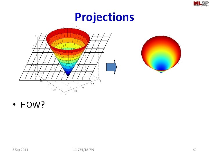
Projections • HOW? 2 Sep 2014 11 -755/18 -797 62

Projections • Draw any two vectors W 1 and W 2 that lie on the plane – ANY two so long as they have different angles • • Compose a matrix W = [W 1 W 2] Compose the projection matrix P = W (WTW)-1 WT Multiply every point on the cone by P to get its projection View it – I’m missing a step here – what is it? 2 Sep 2014 11 -755/18 -797 63

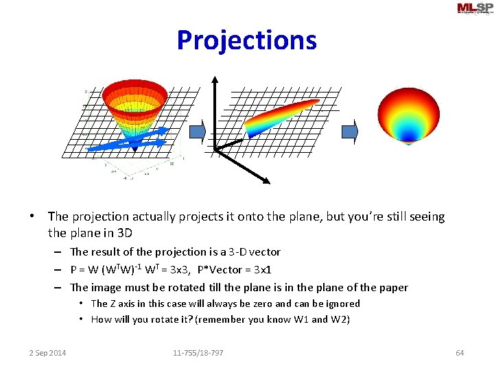
Projections • The projection actually projects it onto the plane, but you’re still seeing the plane in 3 D – The result of the projection is a 3 -D vector – P = W (WTW)-1 WT = 3 x 3, P*Vector = 3 x 1 – The image must be rotated till the plane is in the plane of the paper • The Z axis in this case will always be zero and can be ignored • How will you rotate it? (remember you know W 1 and W 2) 2 Sep 2014 11 -755/18 -797 64

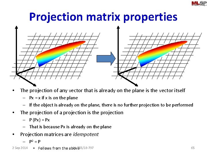
Projection matrix properties • The projection of any vector that is already on the plane is the vector itself – Px = x if x is on the plane – If the object is already on the plane, there is no further projection to be performed • The projection of a projection is the projection – P (Px) = Px – That is because Px is already on the plane • Projection matrices are idempotent – P 2 = P 2 Sep 2014 11 -755/18 -797 • Follows from the above 65

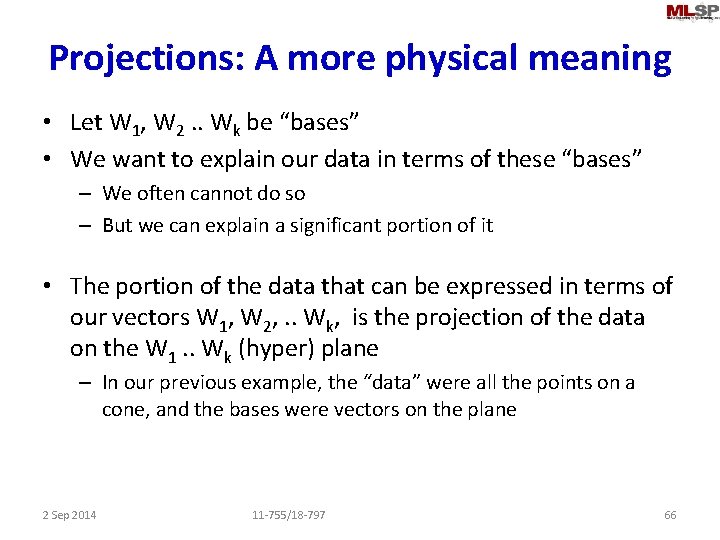
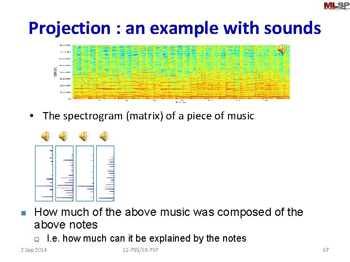
Projections: A more physical meaning • Let W 1, W 2. . Wk be “bases” • We want to explain our data in terms of these “bases” – We often cannot do so – But we can explain a significant portion of it • The portion of the data that can be expressed in terms of our vectors W 1, W 2, . . Wk, is the projection of the data on the W 1. . Wk (hyper) plane – In our previous example, the “data” were all the points on a cone, and the bases were vectors on the plane 2 Sep 2014 11 -755/18 -797 66

Projection : an example with sounds • The spectrogram (matrix) of a piece of music n How much of the above music was composed of the above notes q I. e. how much can it be explained by the notes 2 Sep 2014 11 -755/18 -797 67

Projection: one note M= • The spectrogram (matrix) of a piece of music W= M = spectrogram; W = note n P = W (WTW)-1 WT n Projected Spectrogram = P * M 2 Sep 2014 11 -755/18 -797 n 68

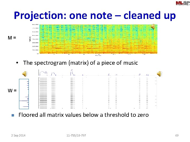
Projection: one note – cleaned up M= • The spectrogram (matrix) of a piece of music W= n Floored all matrix values below a threshold to zero 2 Sep 2014 11 -755/18 -797 69

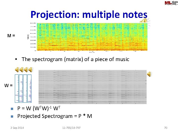
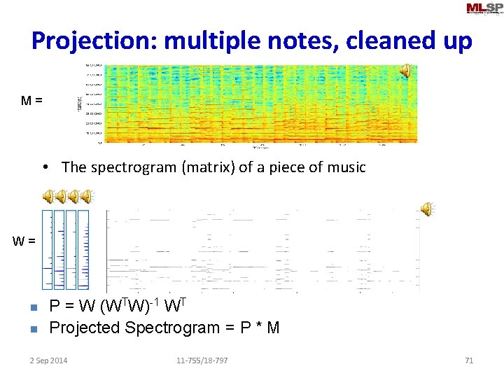
Projection: multiple notes M= • The spectrogram (matrix) of a piece of music W= n n P = W (WTW)-1 WT Projected Spectrogram = P * M 2 Sep 2014 11 -755/18 -797 70

Projection: multiple notes, cleaned up M= • The spectrogram (matrix) of a piece of music W= n n P = W (WTW)-1 WT Projected Spectrogram = P * M 2 Sep 2014 11 -755/18 -797 71

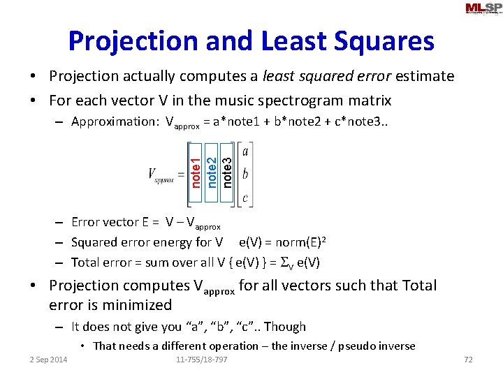
Projection and Least Squares • Projection actually computes a least squared error estimate • For each vector V in the music spectrogram matrix note 1 note 2 note 3 – Approximation: Vapprox = a*note 1 + b*note 2 + c*note 3. . – Error vector E = V – Vapprox – Squared error energy for V e(V) = norm(E)2 – Total error = sum over all V { e(V) } = SV e(V) • Projection computes Vapprox for all vectors such that Total error is minimized – It does not give you “a”, “b”, “c”. . Though • That needs a different operation – the inverse / pseudo inverse 2 Sep 2014 11 -755/18 -797 72

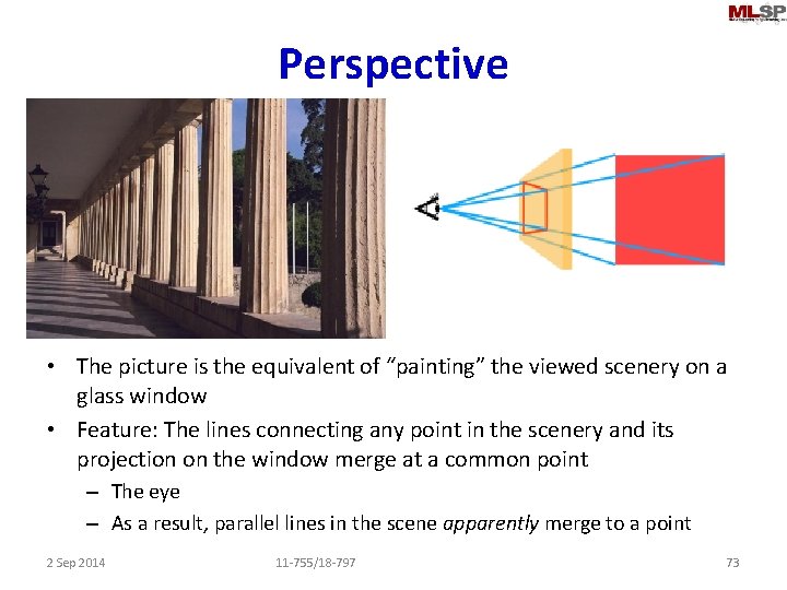
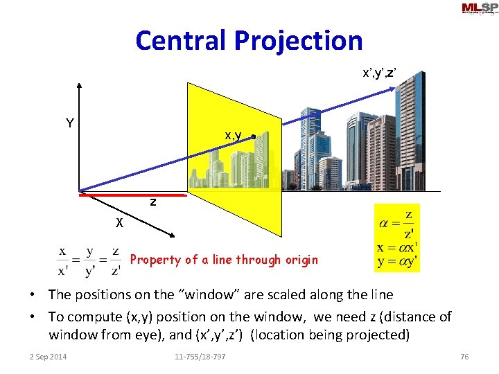
Perspective • The picture is the equivalent of “painting” the viewed scenery on a glass window • Feature: The lines connecting any point in the scenery and its projection on the window merge at a common point – The eye – As a result, parallel lines in the scene apparently merge to a point 2 Sep 2014 11 -755/18 -797 73

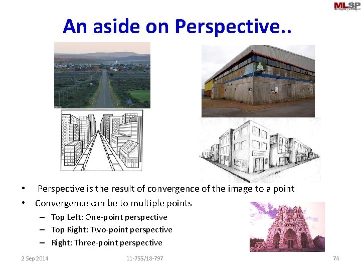
An aside on Perspective. . • Perspective is the result of convergence of the image to a point • Convergence can be to multiple points – Top Left: One-point perspective – Top Right: Two-point perspective – Right: Three-point perspective 2 Sep 2014 11 -755/18 -797 74

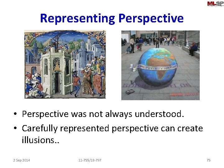
Representing Perspective • Perspective was not always understood. • Carefully represented perspective can create illusions. . 2 Sep 2014 11 -755/18 -797 75

Central Projection x’, y’, z’ Y x, y z X Property of a line through origin • The positions on the “window” are scaled along the line • To compute (x, y) position on the window, we need z (distance of window from eye), and (x’, y’, z’) (location being projected) 2 Sep 2014 11 -755/18 -797 76

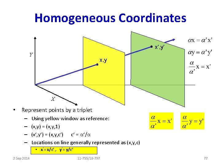
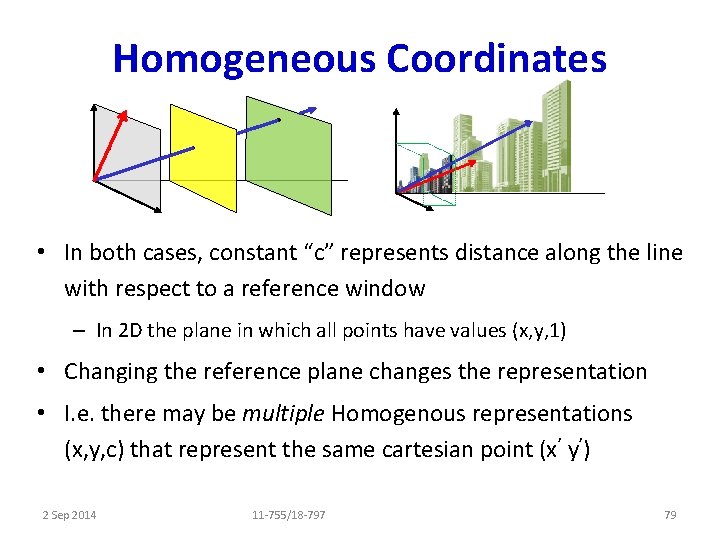
Homogeneous Coordinates x’, y’ Y x, y X • Represent points by a triplet – – Using yellow window as reference: (x, y) = (x, y, 1) (x’, y’) = (x, y, c’) c’ = a’/a Locations on line generally represented as (x, y, c) • x’= x/c’ , y’= y/c’ 2 Sep 2014 11 -755/18 -797 77

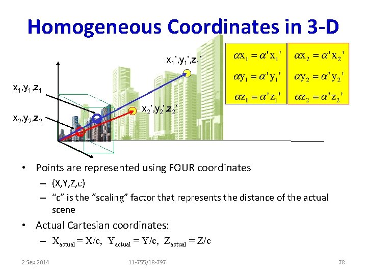
Homogeneous Coordinates in 3 -D x 1’, y 1’, z 1’ x 1, y 1, z 1 x 2, y 2, z 2 x 2’, y 2’, z 2’ • Points are represented using FOUR coordinates – (X, Y, Z, c) – “c” is the “scaling” factor that represents the distance of the actual scene • Actual Cartesian coordinates: – Xactual = X/c, Yactual = Y/c, Zactual = Z/c 2 Sep 2014 11 -755/18 -797 78

Homogeneous Coordinates • In both cases, constant “c” represents distance along the line with respect to a reference window – In 2 D the plane in which all points have values (x, y, 1) • Changing the reference plane changes the representation • I. e. there may be multiple Homogenous representations (x, y, c) that represent the same cartesian point (x’ y’) 2 Sep 2014 11 -755/18 -797 79