Machine Learning for Cyber Unit Linear Regression in

Learning Outcomes Upon completion of this unit: • Students will have a better understanding of linear regression in Tensor. Flow • Basic theory of linear regression algorithm • Tensor. Flow • mechanics This document is licensed with a Creative Commons Attribution 4. 0 International License © 2017

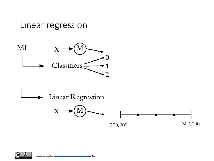
Linear regression 0 1 2 200, 000 This document is licensed with a Creative

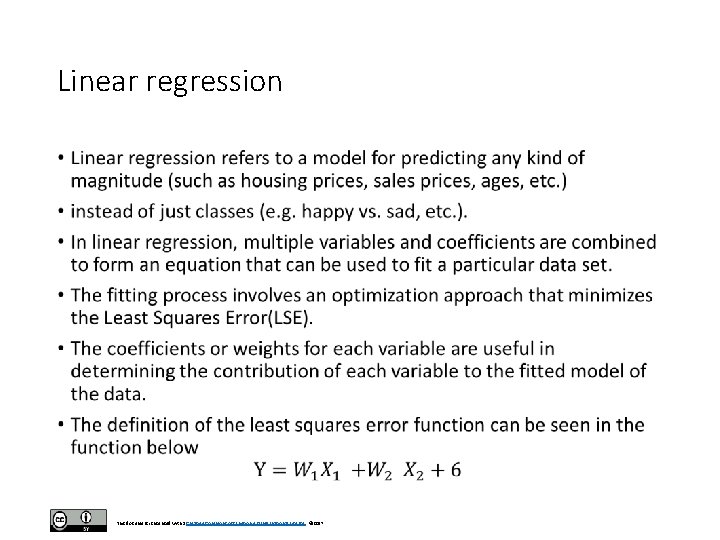
Linear regression • This document is licensed with a Creative Commons Attribution 4. 0

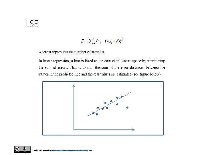
LSE This document is licensed with a Creative Commons Attribution 4. 0 International License

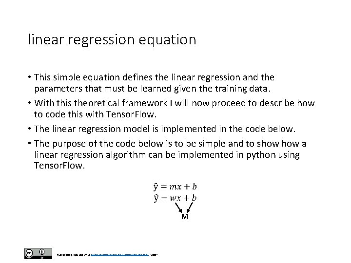
linear regression equation • This simple equation defines the linear regression and the parameters that must be learned given the training data. • With this theoretical framework I will now proceed to describe how to code this with Tensor. Flow. • The linear regression model is implemented in the code below. • The purpose of the code below is to be simple and to show a linear regression algorithm can be implemented in python using Tensor. Flow. M This document is licensed with a Creative Commons Attribution 4. 0 International License © 2017

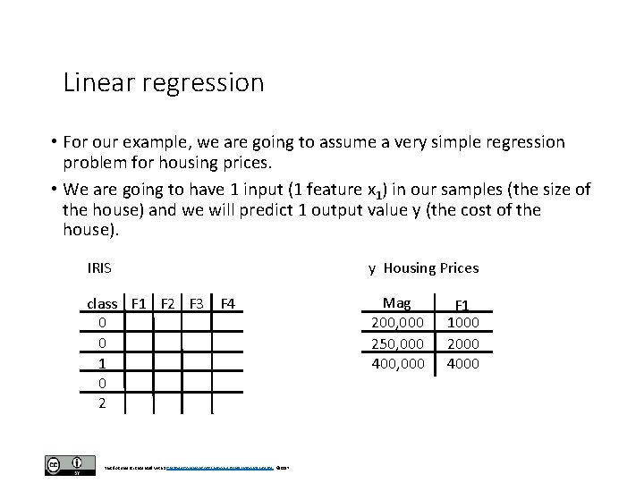
Linear regression • For our example, we are going to assume a very simple regression problem for housing prices. • We are going to have 1 input (1 feature x 1) in our samples (the size of the house) and we will predict 1 output value y (the cost of the house). IRIS y Housing Prices class F 1 F 2 F 3 F 4 0 0 1 0 2 Mag 200, 000 250, 000 400, 000 This document is licensed with a Creative Commons Attribution 4. 0 International License © 2017 F 1 1000 2000 4000

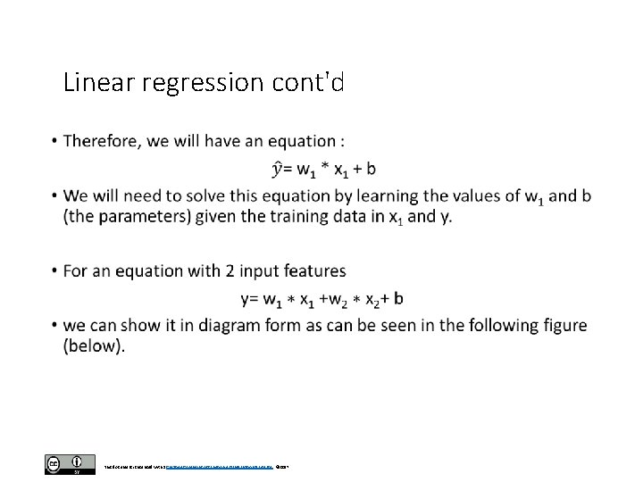
Linear regression cont'd • This document is licensed with a Creative Commons Attribution 4.

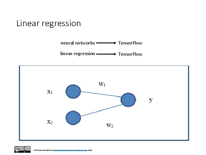
Linear regression neural networks Tensor. Flow linear regression Tensor. Flow This document is licensed

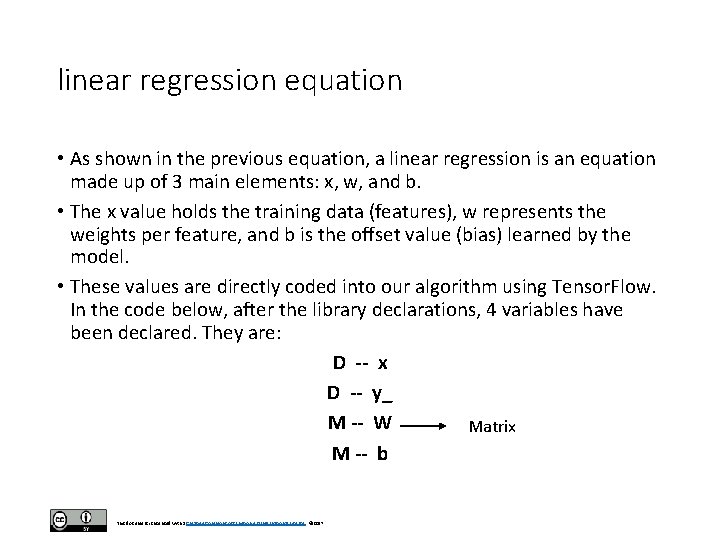
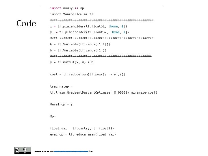
linear regression equation • As shown in the previous equation, a linear regression is an equation made up of 3 main elements: x, w, and b. • The x value holds the training data (features), w represents the weights per feature, and b is the offset value (bias) learned by the model. • These values are directly coded into our algorithm using Tensor. Flow. In the code below, after the library declarations, 4 variables have been declared. They are: D -- x D -- y_ M -- W Matrix M -- b This document is licensed with a Creative Commons Attribution 4. 0 International License © 2017

Code 1 2 3 4 This document is licensed with a Creative Commons Attribution

Session This document is licensed with a Creative Commons Attribution 4. 0 International License

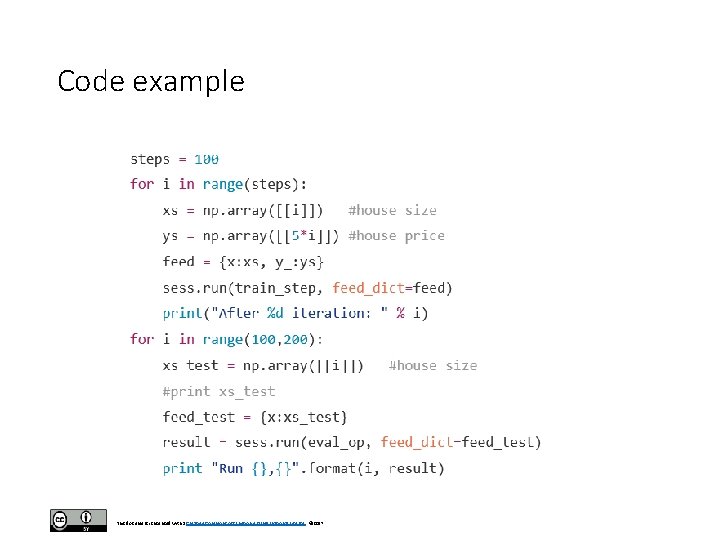
Code example This document is licensed with a Creative Commons Attribution 4. 0 International

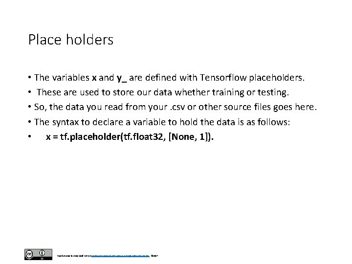
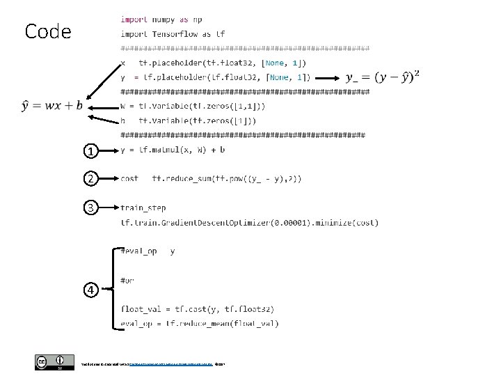
Place holders • The variables x and y_ are defined with Tensorflow placeholders. • These are used to store our data whether training or testing. • So, the data you read from your. csv or other source files goes here. • The syntax to declare a variable to hold the data is as follows: • x = tf. placeholder(tf. float 32, [None, 1]). This document is licensed with a Creative Commons Attribution 4. 0 International License © 2017

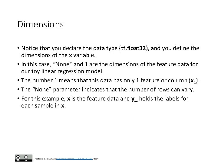
Dimensions • Notice that you declare the data type (tf. float 32), and you define the dimensions of the x variable. • In this case, “None” and 1 are the dimensions of the feature data for our toy linear regression model. • The number 1 means that this data has only 1 feature or column (x 1). • The “None” parameter indicates that the number of rows can vary. • For this example, x is the feature data and y_ holds the labels for each sample in x. This document is licensed with a Creative Commons Attribution 4. 0 International License © 2017

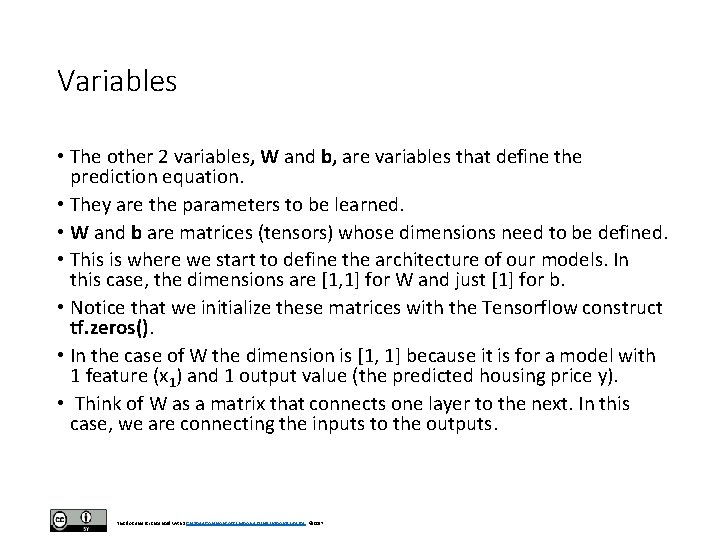
Variables • The other 2 variables, W and b, are variables that define the prediction equation. • They are the parameters to be learned. • W and b are matrices (tensors) whose dimensions need to be defined. • This is where we start to define the architecture of our models. In this case, the dimensions are [1, 1] for W and just [1] for b. • Notice that we initialize these matrices with the Tensorflow construct tf. zeros(). • In the case of W the dimension is [1, 1] because it is for a model with 1 feature (x 1) and 1 output value (the predicted housing price y). • Think of W as a matrix that connects one layer to the next. In this case, we are connecting the inputs to the outputs. This document is licensed with a Creative Commons Attribution 4. 0 International License © 2017

eval_op • In the previous code, the statement eval_op = tf. reduce_mean(float_val) • is used because there is only one value in the tensor. • For example [[996. 23]] and the function tf. reduce_mean() returns just the value 996. 23 (i. e. without the square brackets). • The function tf. reduce_mean() is a built in Tensorflow function that takes as input a tensor and computes the mean of the elements across the dimensions of a given tensor. • So, it returns a reduced tensor. This document is licensed with a Creative Commons Attribution 4. 0 International License © 2017

tf. reduce_mean() • For example, given: x = tf. constant( [[1, 1] , [2, 2]] ) • we can get the following: all = tf. reduce_mean(x) => # 1. 5 all = tf. reduce_mean(x, 0) => # [1. 5, 1. 5] all = tf. reduce_mean(x, 1) => # [1, 2] • To see the results, we can run: print sess. run(all) This document is licensed with a Creative Commons Attribution 4. 0 International License © 2017

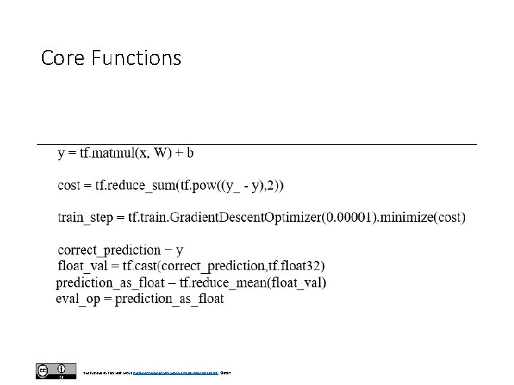
Core Functions • Okay, so now that we have defined the variables, the next step is to define the equation and define the cost function to learn the parameters (e. g. the weights). • To do that, we use the following section of code. • This is one of the most important parts of deep learning programming. • I also want to emphasize that the code in the segment below is the section that will vary the most for the different models. • That is, this is where we define the specifics of the linear regression model, or the logistic regression model, or the neural network model, or the deep neural network model. • In essence, this is the heart or core of it all or is it the brains? This document is licensed with a Creative Commons Attribution 4. 0 International License © 2017

Core Functions This document is licensed with a Creative Commons Attribution 4. 0 International

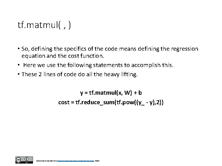
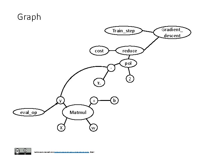
tf. matmul( , ) • So, defining the specifics of the code means defining the regression equation and the cost function. • Here we use the following statements to accomplish this. • These 2 lines of code do all the heavy lifting. y = tf. matmul(x, W) + b cost = tf. reduce_sum(tf. pow((y_ - y), 2)) This document is licensed with a Creative Commons Attribution 4. 0 International License © 2017

tf. matmul() • The first statement y = tf. matmul(x, W) + b defines the regression equation. • We use tf. matmul(x, W) to perform the matrix multiplication and we add b to the result. • The dimensions of the b vector need to match the dimension of the j index of the weights vector (weights=[i, j]). • As a side note, I will point out here that Tensorflow is designed to be used with GPUs, and GPUs are very good at matrix multiplications. • The function tf. matmul() will perform these multiplications. This is the power of Tensorflow. This document is licensed with a Creative Commons Attribution 4. 0 International License © 2017

Cost • The line cost = tf. reduce_sum(tf. pow((y_ - y), 2)) defines the cost function. • This is the standard least squares cost function in linear regression. • Notice that the tf. pow() function raises the difference between vector y_ and vector y to the power of 2. • This result is passed through the tf. reduce_sum() function and assigned to cost. • The function tf. reduce_sum() computes the sum of the elements across dimensions of a tensor. This document is licensed with a Creative Commons Attribution 4. 0 International License © 2017

tf. reduce_sum() >>>x = tf. constant( [[1, 1, 1], [1, 1, 1]]) >>>y = tf. reduce_sum(x) #6 >>>y = tf. reduce_sum(x, 0) #[2, 2, 2] >>>y = tf. reduce_sum(x, 1) #[3, 3] This document is licensed with a Creative Commons Attribution 4. 0 International License © 2017

Gradient Descent • Whenever we want to reference the cost function or the regression equation, we can just do so by the variable names we defined for them which are y and cost, in this case. • Once the cost function is defined, we need to tell the model what optimization to use. In this case, the line: train_step=tf. train. Gradient. Descent. Optimizer(0. 00001). minimize (cost) • indicates that we should use a gradient descent optimizer with a step size of 0. 00001. This document is licensed with a Creative Commons Attribution 4. 0 International License © 2017

train_step • This object, train_step, is now the optimizer which references the cost function via cost. • And cost itself is linked to the regression equation via y. • The final part of this code segment just takes the predicted y value and performs typecasting and reducing operations (e. g. if you have a vector of values, average all of them and return 1 averaged value). This document is licensed with a Creative Commons Attribution 4. 0 International License © 2017

Graph Train_step reduce cost pol - 2 y_ y + Matmul eval_op X w

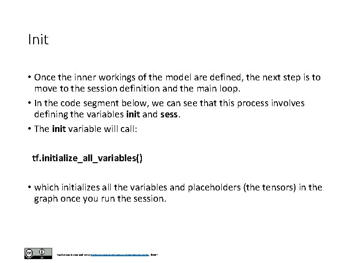
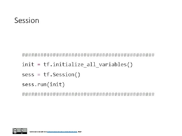
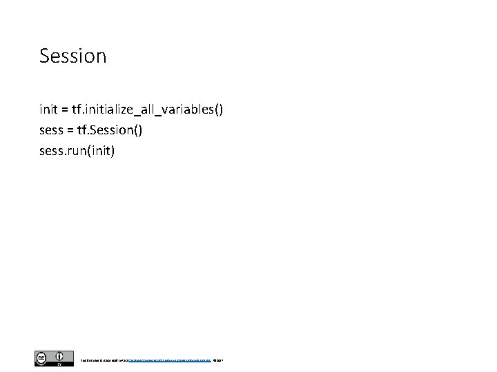
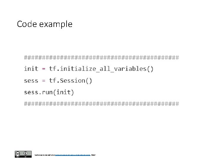
Init • Once the inner workings of the model are defined, the next step is to move to the session definition and the main loop. • In the code segment below, we can see that this process involves defining the variables init and sess. • The init variable will call: tf. initialize_all_variables() • which initializes all the variables and placeholders (the tensors) in the graph once you run the session. This document is licensed with a Creative Commons Attribution 4. 0 International License © 2017

sess. run() • Consider that at this point all we have done is define the graph structure without actually running anything in Tensorflow. • To run things in Tensorflow we use sess. run() with the variable we want to run it with. • In this case, we want to initialize the variables so we run sess. run(init). This document is licensed with a Creative Commons Attribution 4. 0 International License © 2017

Session init = tf. initialize_all_variables() sess = tf. Session() sess. run(init) This document is

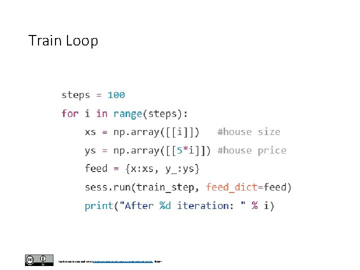
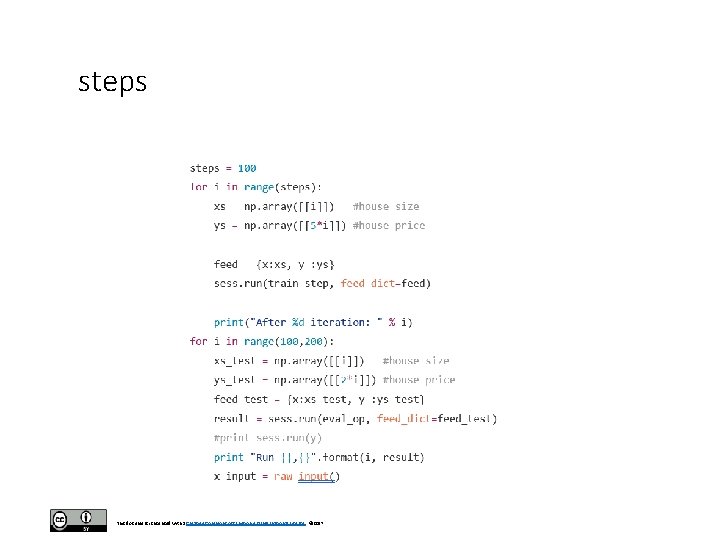
Main Loop • Finally, the last part in our linear regression code is to run the main loop to actually train and test the model. • In this case, I have broken up the main loop into 2 separate loops for better visualization. • The first loop is for training and the second loop is for testing. The first training loop is very simple. • The training data, in this case, is not read from a file but instead is created automatically. • The feature vector is stored in xs and contains only one feature (x 1) which is the “i” index. • This feature represents the size of the house. • The corresponding housing price for each xs sample is stored in ys. This document is licensed with a Creative Commons Attribution 4. 0 International License © 2017

housing price example • For this scenario, each housing price value is 5 times its corresponding house size. • Therefore, our model after training should be equivalent to: • y = 5 * x 1 + b. • In this case, the training phase would optimize the weight vector to be equal to 5 (W 1=5). • Notice that the process is repeated 100 times. • Once xs and ys are defined, these values are assigned to the feed dictionary. • This is an internal mechanism of Tensorflow that is very useful f • or passing the data from the python code to the Tensorflow graph. In this case, xs is assigned to x and ys is assigned to y_. • These variables are the same ones that we have already defined in the code. This document is licensed with a Creative Commons Attribution 4. 0 International License © 2017

sess. run(train_step) • The last part is to run the graph. Finally, this is where your Tensorflow code will run. • Before now, the code had not executed but after sess. run(train_step), the code finally executes. • In this case we run train_step and everything that is linked to train_step. • So we run the gradient descent optimizer, the cost function for least squares estimation, and the linear regression equation. This document is licensed with a Creative Commons Attribution 4. 0 International License © 2017

Train Loop This document is licensed with a Creative Commons Attribution 4. 0 International

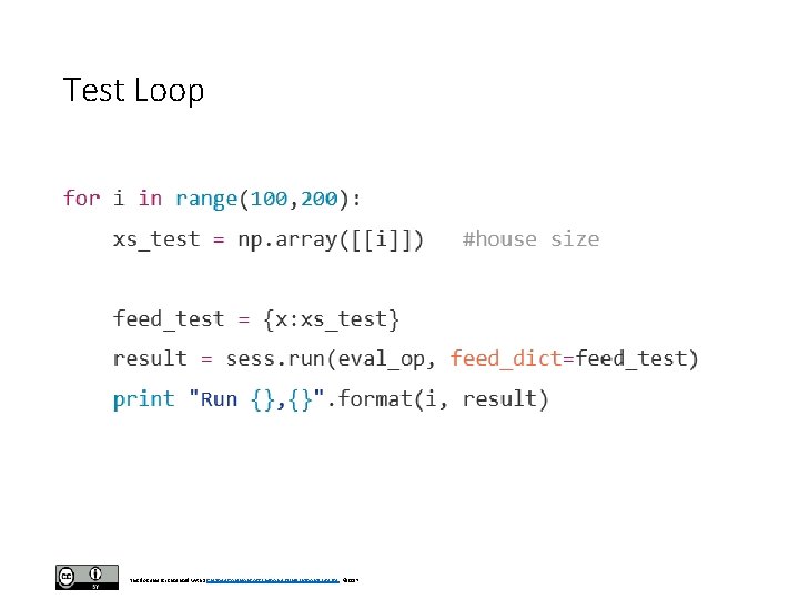
The second loop • The second loop (below) is very similar to the first one except that it is focused on the testing phase. • Here we use the model from the training phase to predict the housing prices given the house sizes for the range of values from 100 to 200. • Remember that the data is created automatically, for this example. Notice that sess. run() now calls eval_op. • The variable eval_op is linked to y which is basically the linear regression model. This document is licensed with a Creative Commons Attribution 4. 0 International License © 2017

Test Loop This document is licensed with a Creative Commons Attribution 4. 0 International

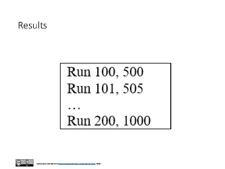
xs_test • So, here we used the trained model but with a new dataset xs_test. • The result is stored in the variable result and printed out on the screen. • The result of the classification should be that the regression model predicts housing prices that are 5 times the input house size. • This outcome can be seen in the output below. This document is licensed with a Creative Commons Attribution 4. 0 International License © 2017

Results This document is licensed with a Creative Commons Attribution 4. 0 International License

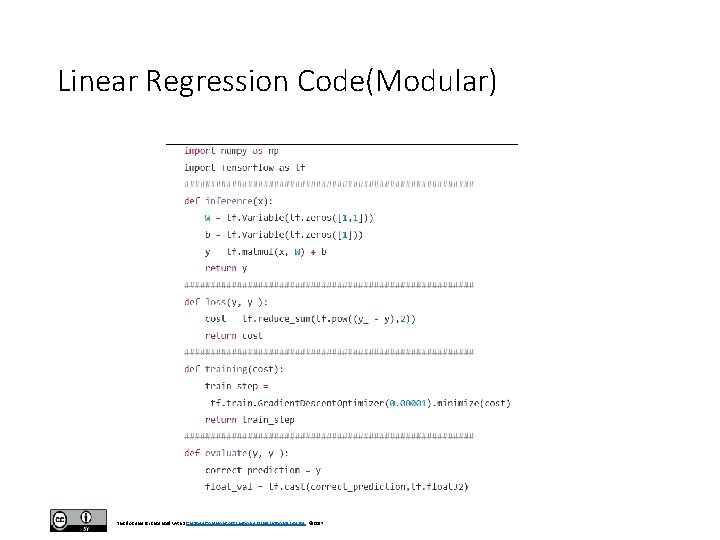
Modular Approach • The previous code for linear regression can be re-written in a more modular form using function calls. • This approach will be very helpful later on as most implementations can be written in the same way and the only thing that changes is the internal definition of the functions. • This new modular approach can be seen next. This document is licensed with a Creative Commons Attribution 4. 0 International License © 2017

Code This document is licensed with a Creative Commons Attribution 4. 0 International License

Linear Regression Code(Modular) This document is licensed with a Creative Commons Attribution 4. 0

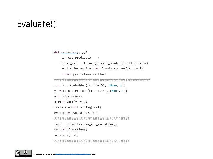
Evaluate() This document is licensed with a Creative Commons Attribution 4. 0 International License

steps This document is licensed with a Creative Commons Attribution 4. 0 International License

Wrap up • As can be seen from the previous code example, not much had to change in the code to make it more readable, modular, and easier to modify. • The new aspects are that we now have 4 functions that can be used to define the model. • They are: • • inference() for the equation loss( ) for the cost function training() for the optimization evaluate() for the performance estimation This document is licensed with a Creative Commons Attribution 4. 0 International License © 2017

Summary • We discussed linear regression in Tensor. Flow v Tensor. Flow code v Linear Regression theory Tensor. Flow v Graph <=code v Modular approach Lin R Log R NN DNN This document is licensed with a Creative Commons Attribution 4. 0 International License © 2017