Machine Learning For Cyber Unit 12 Logistic Regression
Machine Learning For Cyber Unit 12: Logistic Regression in Tensor. Flow This document is licensed with a Creative Commons Attribution 4. 0 International License © 2017
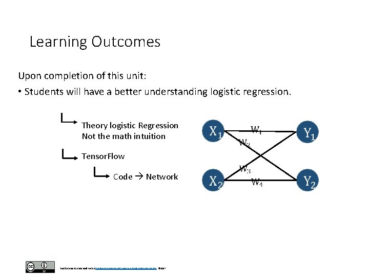
Learning Outcomes Upon completion of this unit: • Students will have a better understanding logistic regression. Theory logistic Regression Not the math intuition Tensor. Flow Code Network This document is licensed with a Creative Commons Attribution 4. 0 International License © 2017
Terms • Logistic regression • Tensor. Flow This document is licensed with a Creative Commons Attribution 4. 0 International License © 2017
Neural Nets • Before we look at the deep neural nets, it is a good idea to look at logistic regression. • Logistic regression is still a linear classifier but deep neural nets can build on the ideas of logistic regression. • So, basically here we will use all the code we have developed so far. • The only difference is that now we will re-define the code for the functions: inference() loss() • As we can see in the next code segment, inference is mainly different from the linear regression approach because we now run our equation tf. matmul(x_tf, W) + b This document is licensed with a Creative Commons Attribution 4. 0 International License © 2017
Softmax Function • through a softmax function. • Additionally, instead of predicting a real valued number with just one output neuron, we now have several output neurons which represent each possible class (3 in the case of IRIS, or 10 in the case of MNIST). • Intuitively think of it this way. This document is licensed with a Creative Commons Attribution 4. 0 International License © 2017
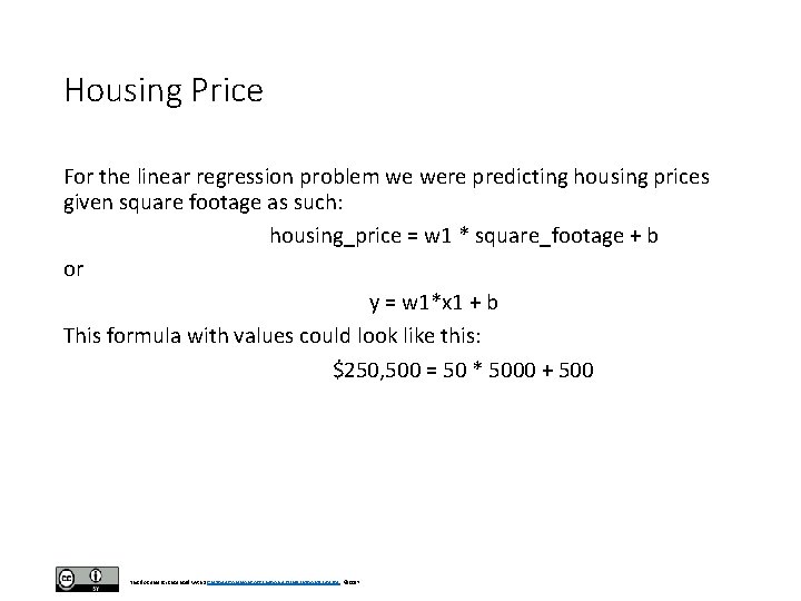
Housing Price For the linear regression problem we were predicting housing prices given square footage as such: housing_price = w 1 * square_footage + b or y = w 1*x 1 + b This formula with values could look like this: $250, 500 = 50 * 5000 + 500 This document is licensed with a Creative Commons Attribution 4. 0 International License © 2017
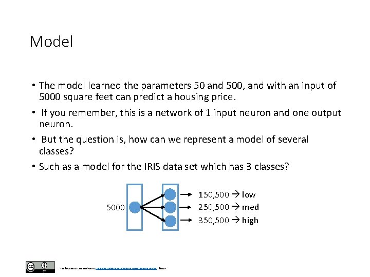
Model • The model learned the parameters 50 and 500, and with an input of 5000 square feet can predict a housing price. • If you remember, this is a network of 1 input neuron and one output neuron. • But the question is, how can we represent a model of several classes? • Such as a model for the IRIS data set which has 3 classes? 5000 This document is licensed with a Creative Commons Attribution 4. 0 International License © 2017 150, 500 low 250, 500 med 350, 500 high
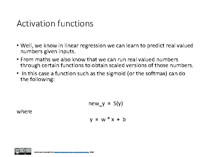
Activation functions • Well, we know in linear regression we can learn to predict real valued numbers given inputs. • From maths we also know that we can run real valued numbers through certain functions to obtain scaled versions of those numbers. • In this case a function such as the sigmoid (or the softmax) can do the following: new_y = S(y) where y = w*x + b This document is licensed with a Creative Commons Attribution 4. 0 International License © 2017
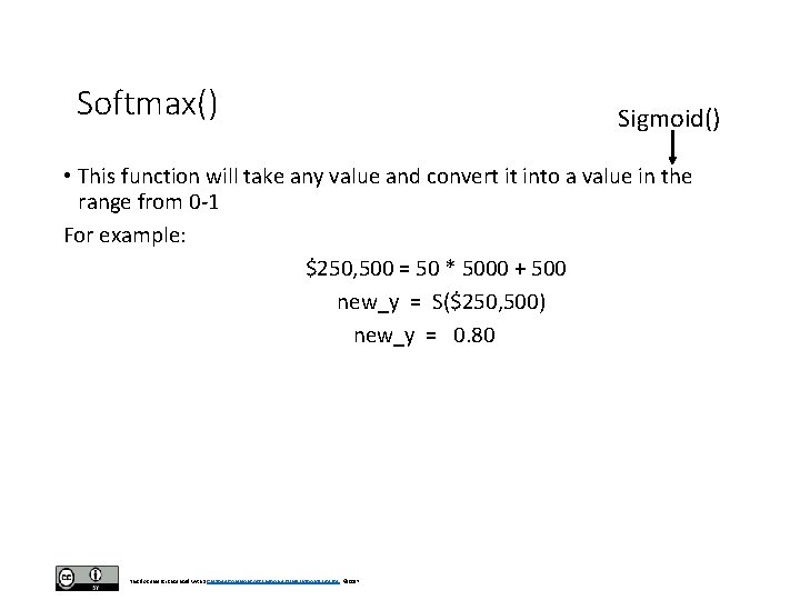
Softmax() Sigmoid() • This function will take any value and convert it into a value in the range from 0 -1 For example: $250, 500 = 50 * 5000 + 500 new_y = S($250, 500) new_y = 0. 80 This document is licensed with a Creative Commons Attribution 4. 0 International License © 2017
Softmax function • So, this allows us to learn functions that predict values between 0 and 1. • This is good because these values can also be interpreted as probabilities or strengths of my prediction. • As in, I have a 0. 80 confidence that the house price is $250, 500. • But what if I had 3 possible housing prices: $150, 700, $250, 500, and $350, 400. • How can I represent this in the previous equation? This document is licensed with a Creative Commons Attribution 4. 0 International License © 2017
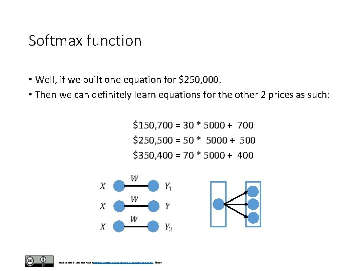
Softmax function • Well, if we built one equation for $250, 000. • Then we can definitely learn equations for the other 2 prices as such: $150, 700 = 30 * 5000 + 700 $250, 500 = 50 * 5000 + 500 $350, 400 = 70 * 5000 + 400 This document is licensed with a Creative Commons Attribution 4. 0 International License © 2017
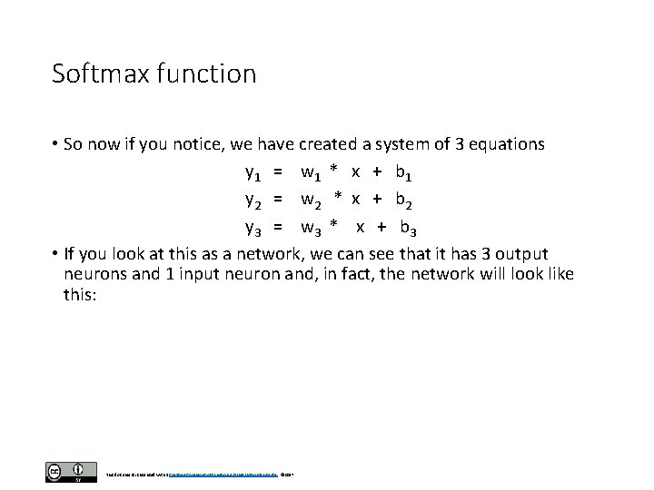
Softmax function • So now if you notice, we have created a system of 3 equations y 1 = w 1 * x + b 1 y 2 = w 2 * x + b 2 y 3 = w 3 * x + b 3 • If you look at this as a network, we can see that it has 3 output neurons and 1 input neuron and, in fact, the network will look like this: This document is licensed with a Creative Commons Attribution 4. 0 International License © 2017
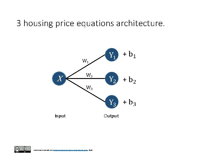
3 housing price equations architecture. X Input This document is licensed with a Creative Commons Attribution 4. 0 International License © 2017 Output
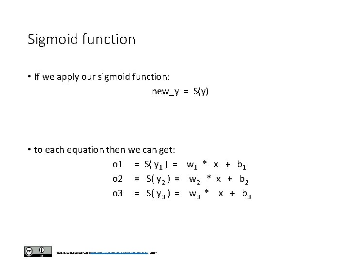
Sigmoid function • If we apply our sigmoid function: new_y = S(y) • to each equation then we can get: o 1 = S( y 1 ) = w 1 * x + b 1 o 2 = S( y 2 ) = w 2 * x + b 2 o 3 = S( y 3 ) = w 3 * x + b 3 This document is licensed with a Creative Commons Attribution 4. 0 International License © 2017
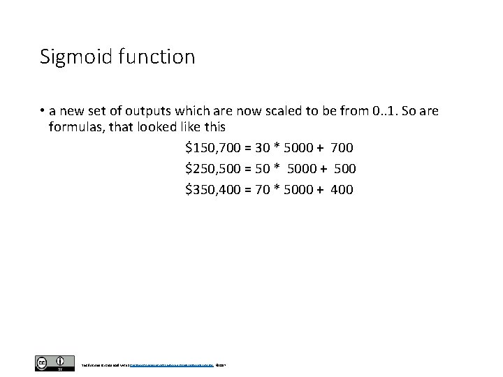
Sigmoid function • a new set of outputs which are now scaled to be from 0. . 1. So are formulas, that looked like this $150, 700 = 30 * 5000 + 700 $250, 500 = 50 * 5000 + 500 $350, 400 = 70 * 5000 + 400 This document is licensed with a Creative Commons Attribution 4. 0 International License © 2017
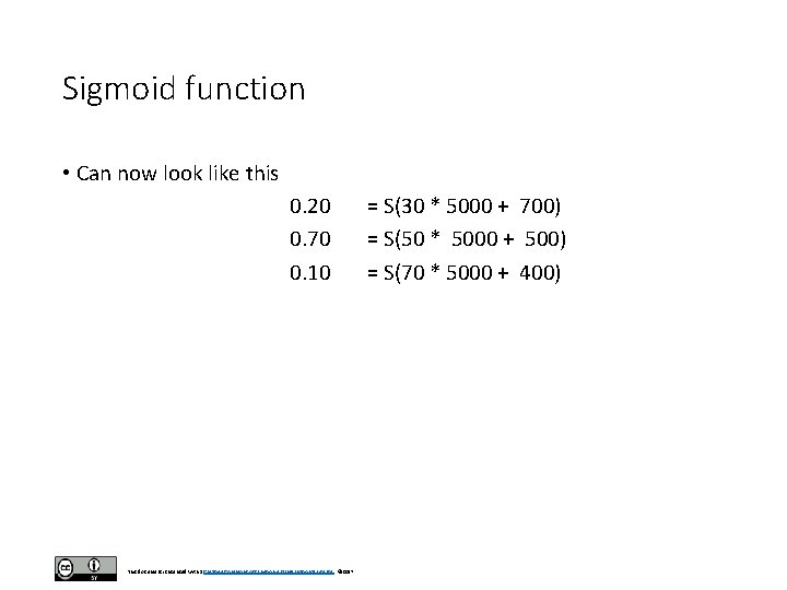
Sigmoid function • Can now look like this 0. 20 0. 70 0. 10 This document is licensed with a Creative Commons Attribution 4. 0 International License © 2017 = S(30 * 5000 + 700) = S(50 * 5000 + 500) = S(70 * 5000 + 400)
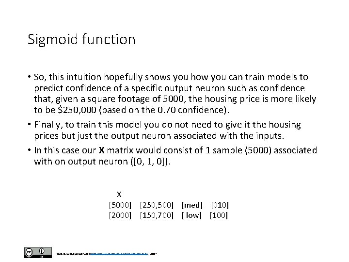
Sigmoid function • So, this intuition hopefully shows you how you can train models to predict confidence of a specific output neuron such as confidence that, given a square footage of 5000, the housing price is more likely to be $250, 000 (based on the 0. 70 confidence). • Finally, to train this model you do not need to give it the housing prices but just the output neuron associated with the inputs. • In this case our X matrix would consist of 1 sample (5000) associated with on output neuron ([0, 1, 0]). X [5000] [250, 500] [med] [010] [2000] [150, 700] [ low] [100] This document is licensed with a Creative Commons Attribution 4. 0 International License © 2017
Softmax() • Formally, a softmax function is a way of mapping a vector of real valued numbers in any range into a vector of real valued numbers in the range of zero to 1 (0 -1. 0) where all the values add up to 1. 0. • The result of the softmax therefore gives a probability distribution over several classes. This document is licensed with a Creative Commons Attribution 4. 0 International License © 2017
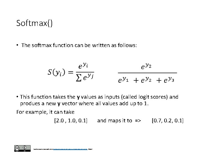
Softmax() • The softmax function can be written as follows: • This function takes the y values as inputs (called logit scores) and produes a new y vector where all values add up to 1. For example, it can take [2. 0 , 1. 0, 0. 1] and maps it to => [0. 7, 0. 2, 0. 1] This document is licensed with a Creative Commons Attribution 4. 0 International License © 2017
![Python (Softmax) >>> logits = [2. 0, 1. 0, 0. 1 ] >>>import numpy Python (Softmax) >>> logits = [2. 0, 1. 0, 0. 1 ] >>>import numpy](http://slidetodoc.com/presentation_image_h2/3bf5a11d4236c8f04d57c907dff45d6e/image-20.jpg)
Python (Softmax) >>> logits = [2. 0, 1. 0, 0. 1 ] >>>import numpy as np >>>exps = [ np. exp(i) for i in logits] >>>sum_of_exps = sum(exp) >>>softmax = [ j/sum_of_exps for j in exps ] >>> print sum(softmax) 1 This document is licensed with a Creative Commons Attribution 4. 0 International License © 2017
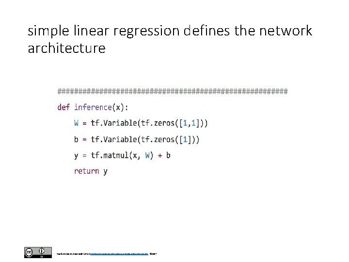
simple linear regression defines the network architecture This document is licensed with a Creative Commons Attribution 4. 0 International License © 2017
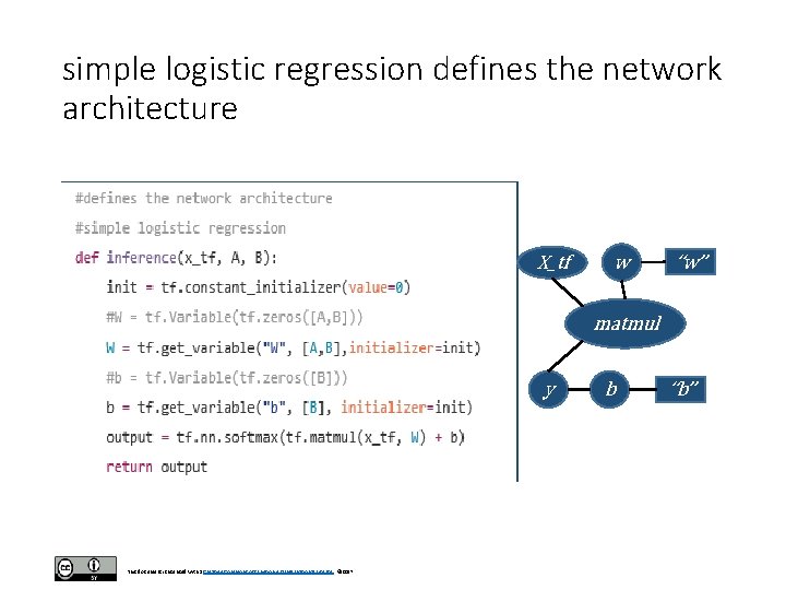
simple logistic regression defines the network architecture X_tf w “w” matmul y This document is licensed with a Creative Commons Attribution 4. 0 International License © 2017 b “b”
tf. get_variable() • Notice that we can use tf. get_variable() instead of tf. Variable() here to declare W and b. The values A and B represent, as previously defined, the number of features and the number of classes. • The difference between tf. Variable() and tf. get_variable() have to do with re-using the same variable. • Basically, tf. Variable() is older and tf. get_variable() is newer and more efficient. • The current Tensorflow world suggestion on this issue is to forget about tf. Variable() and always use tf. get_variable() instead. This document is licensed with a Creative Commons Attribution 4. 0 International License © 2017
iris dataset • So, assuming we are working with the iris dataset, A would be equal to 4 and B would be equal to 3. • The drawing below shows the architecture for a logistic regression model. • If you look closely, you can conclude that a logistic regression model is like a neural network with no hidden layers. • There are only 2 layers: the input layer and the output layer. A hidden layer would be a layer in between input and output that connects these 2 layers. This document is licensed with a Creative Commons Attribution 4. 0 International License © 2017
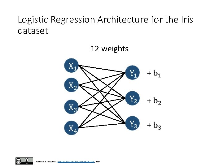
Logistic Regression Architecture for the Iris dataset 12 weights This document is licensed with a Creative Commons Attribution 4. 0 International License © 2017
Code explanation • So for the previous code segment, in W we can see that we create a matrix that is [A, B] in size or for Iris [4, 3]. • The b vector (bias) has dimension B equal to 3 (for the 3 output neurons). • That is, there is now a bias for every neuron in the output layer. • Additionally, notice that the variable init in init = tf. constant_initializer(value=0) helps to initialize Tensorflow variables. This document is licensed with a Creative Commons Attribution 4. 0 International License © 2017
Init: normal distribution • There are several available options in Tensorflow to do this. • Similarly, the loss function is also changed from the linear regression version. • In the linear regression version we used a Least Squares Error loss function. • In this case we now use a logistic regression cost function as shown below. This document is licensed with a Creative Commons Attribution 4. 0 International License © 2017
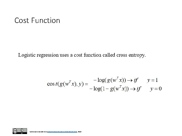
Cost Function This document is licensed with a Creative Commons Attribution 4. 0 International License © 2017
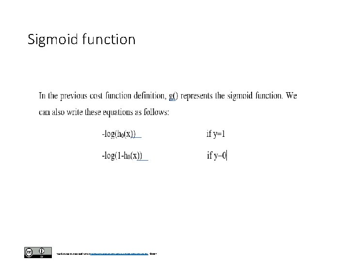
Sigmoid function This document is licensed with a Creative Commons Attribution 4. 0 International License © 2017
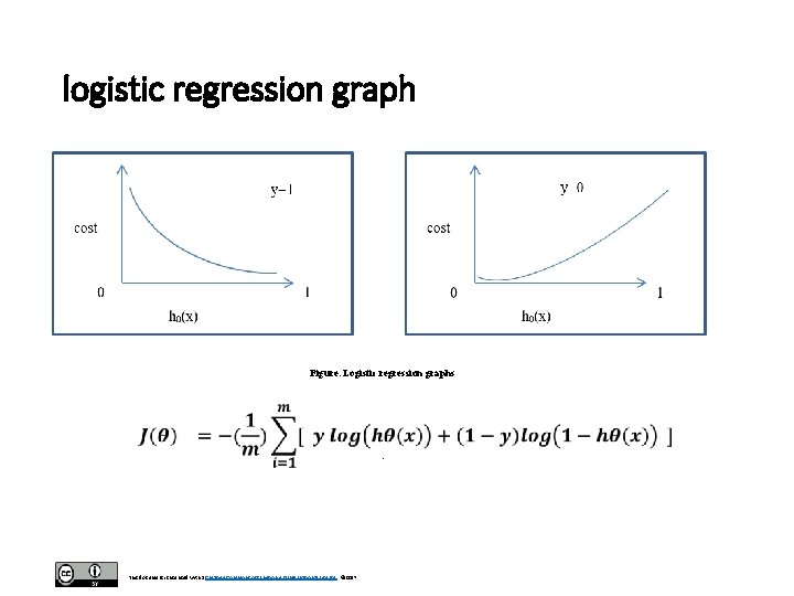
logistic regression graph Figure. Logistic regression graphs . This document is licensed with a Creative Commons Attribution 4. 0 International License © 2017
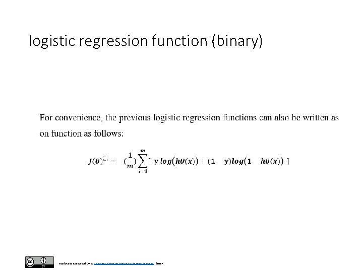
logistic regression function (binary) This document is licensed with a Creative Commons Attribution 4. 0 International License © 2017
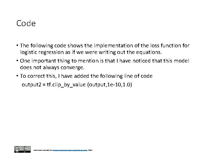
Code • The following code shows the implementation of the loss function for logistic regression as if we were writing out the equations. • One important thing to mention is that I have noticed that this model does not always converge. • To correct this, I have added the following line of code output 2 = tf. clip_by_value (output, 1 e-10, 1. 0) This document is licensed with a Creative Commons Attribution 4. 0 International License © 2017
Clip • This line of code helps because some values in the process become Na. N (Not a number) and the clipping in the function addresses the problem. • This approach of writing out the cost function or equations is not always the most optimal but I have shown it here for contrast between linear regression and logistic regression. • A better approach is to use Tensorflow built-in cost functions for cross entropy calculations. • Future code for deep neural networks will abstract this by using the built-in functions. This document is licensed with a Creative Commons Attribution 4. 0 International License © 2017
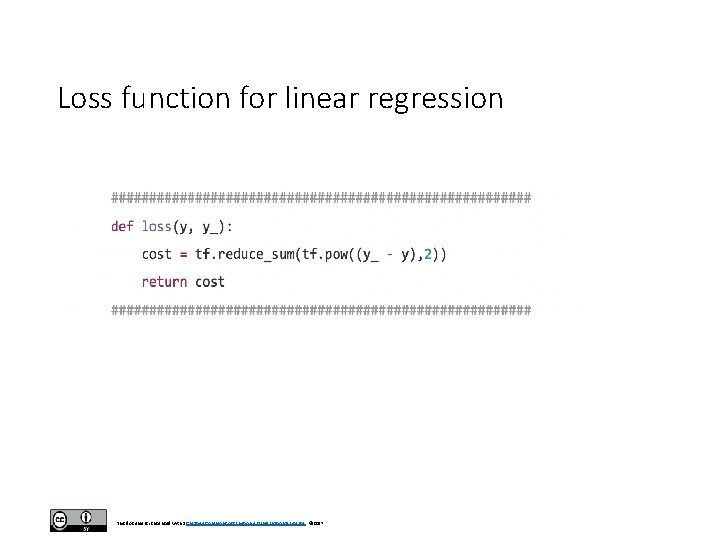
Loss function for linear regression This document is licensed with a Creative Commons Attribution 4. 0 International License © 2017
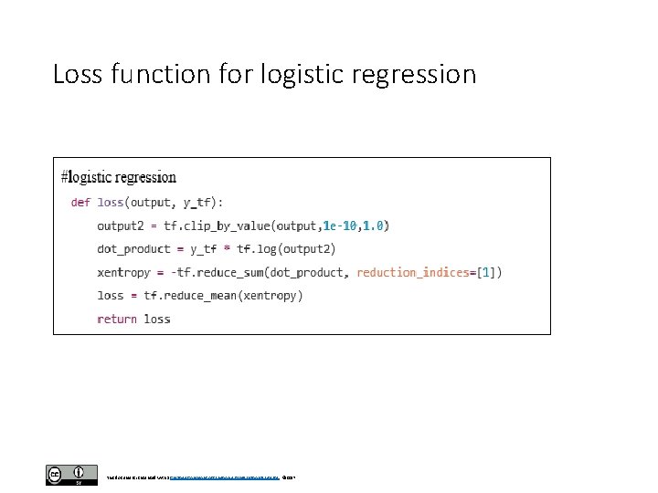
Loss function for logistic regression This document is licensed with a Creative Commons Attribution 4. 0 International License © 2017
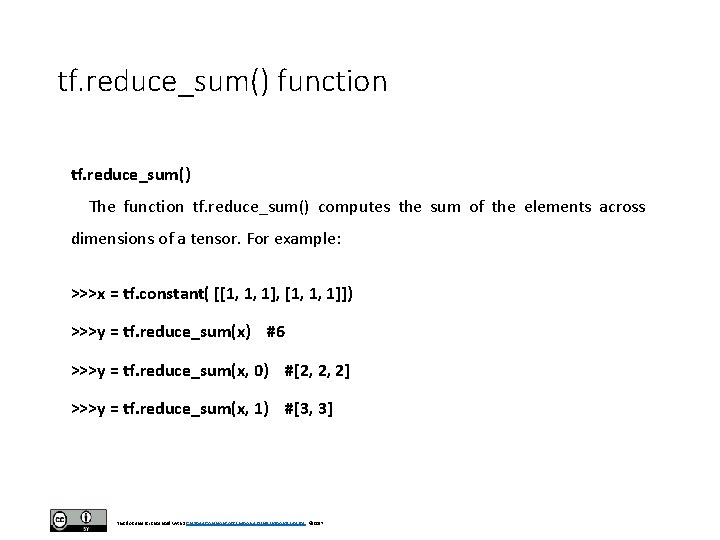
tf. reduce_sum() function tf. reduce_sum() The function tf. reduce_sum() computes the sum of the elements across dimensions of a tensor. For example: >>>x = tf. constant( [[1, 1, 1], [1, 1, 1]]) >>>y = tf. reduce_sum(x) #6 >>>y = tf. reduce_sum(x, 0) #[2, 2, 2] >>>y = tf. reduce_sum(x, 1) #[3, 3] This document is licensed with a Creative Commons Attribution 4. 0 International License © 2017
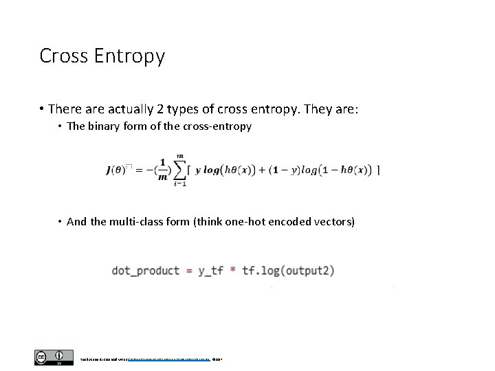
Cross Entropy • There actually 2 types of cross entropy. They are: • The binary form of the cross-entropy • And the multi-class form (think one-hot encoded vectors) This document is licensed with a Creative Commons Attribution 4. 0 International License © 2017
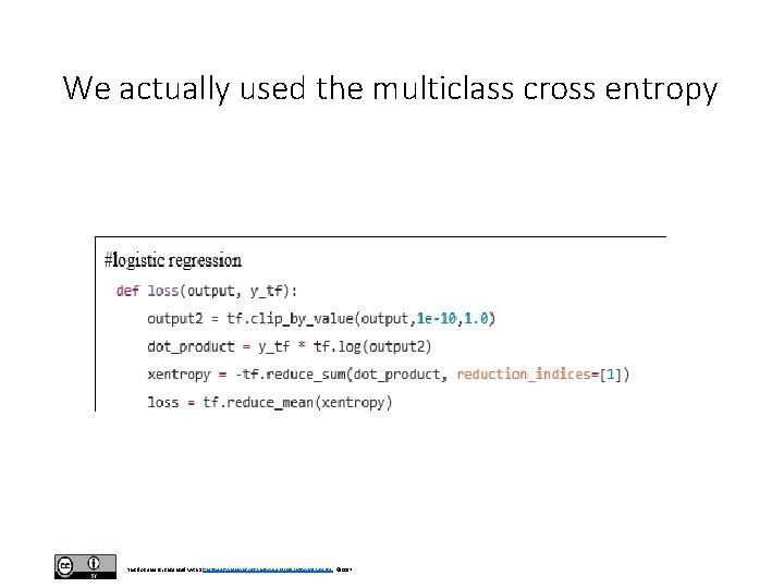
We actually used the multiclass cross entropy This document is licensed with a Creative Commons Attribution 4. 0 International License © 2017
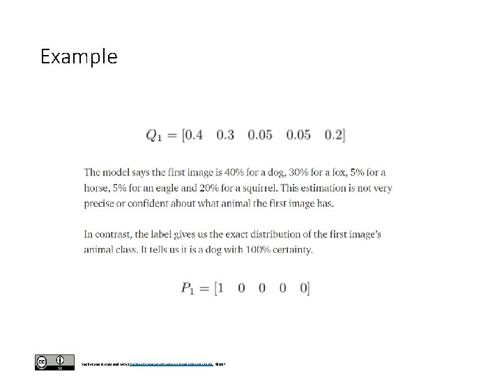
Example This document is licensed with a Creative Commons Attribution 4. 0 International License © 2017
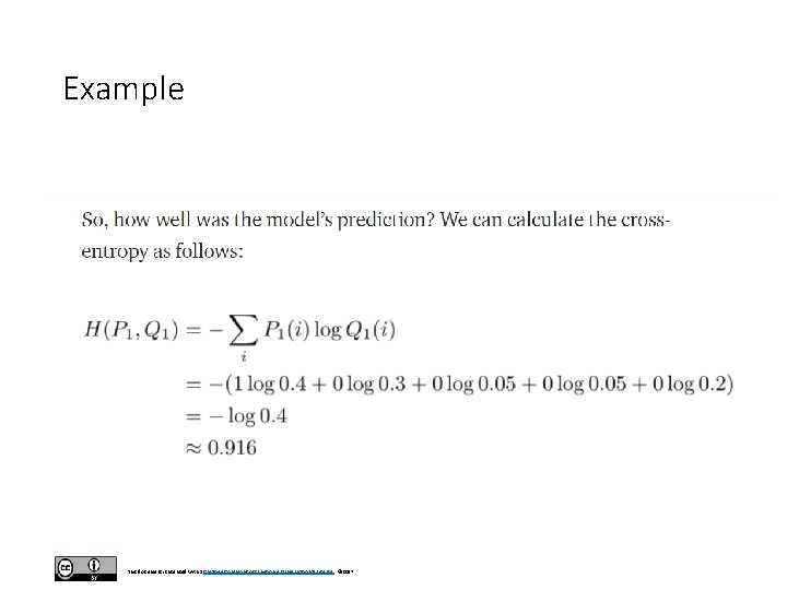
Example This document is licensed with a Creative Commons Attribution 4. 0 International License © 2017
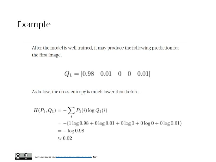
Example This document is licensed with a Creative Commons Attribution 4. 0 International License © 2017
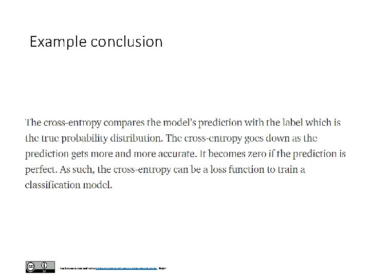
Example conclusion This document is licensed with a Creative Commons Attribution 4. 0 International License © 2017
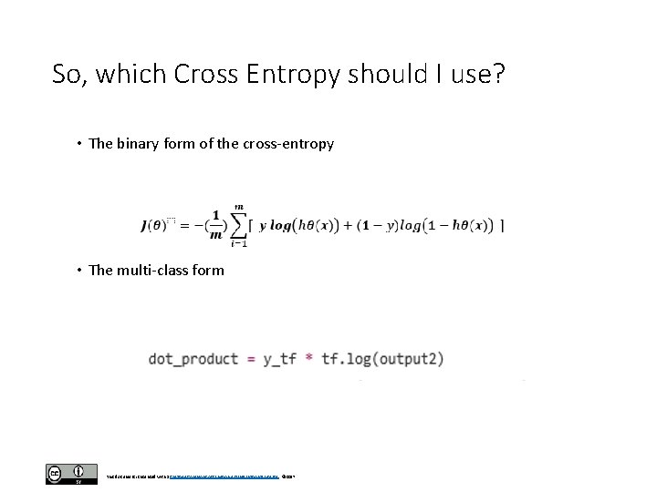
So, which Cross Entropy should I use? • The binary form of the cross-entropy • The multi-class form This document is licensed with a Creative Commons Attribution 4. 0 International License © 2017
Answer: Neither • Instead use: tf. nn. softmax_cross_entropy_with_logits(output, y_tf) • Which is the built in Tensor. Flow cross entropy • When can I use my own loss functions: • • • When you are really sure of what you are doing with loss functions When you understand the numerical methods’ implications of your own loss When you use your own regularization parameters After extensive research When you want to understand intuition for academic growth This document is licensed with a Creative Commons Attribution 4. 0 International License © 2017
Summary • Theory logistic • Linear regression • Logistic regression • Log regression inference() loss() This document is licensed with a Creative Commons Attribution 4. 0 International License © 2017

- Slides: 46