Machine Learning Decision Tree Learning 1 Decision Trees

Machine Learning: Decision Tree Learning 1

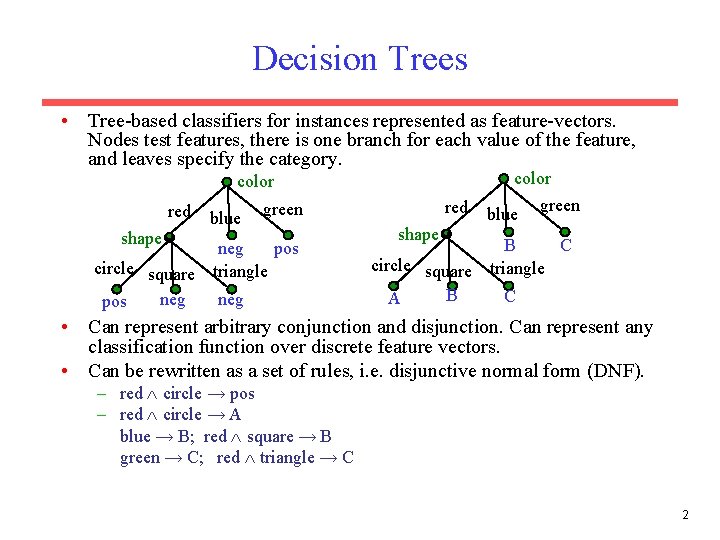
Decision Trees • Tree-based classifiers for instances represented as feature-vectors. Nodes test features, there is one branch for each value of the feature, and leaves specify the category. color red shape blue red green pos neg circle square triangle neg pos shape blue green C B circle square triangle B C A • Can represent arbitrary conjunction and disjunction. Can represent any classification function over discrete feature vectors. • Can be rewritten as a set of rules, i. e. disjunctive normal form (DNF). – red circle → pos – red circle → A blue → B; red square → B green → C; red triangle → C 2

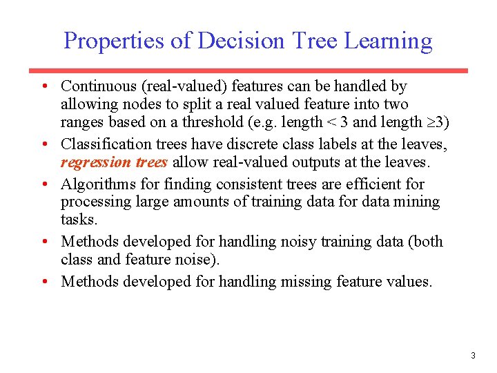
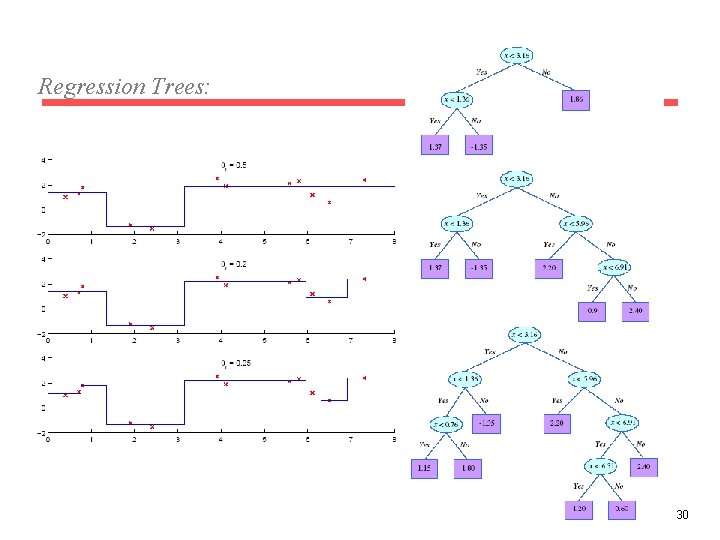
Properties of Decision Tree Learning • Continuous (real-valued) features can be handled by allowing nodes to split a real valued feature into two ranges based on a threshold (e. g. length < 3 and length 3) • Classification trees have discrete class labels at the leaves, regression trees allow real-valued outputs at the leaves. • Algorithms for finding consistent trees are efficient for processing large amounts of training data for data mining tasks. • Methods developed for handling noisy training data (both class and feature noise). • Methods developed for handling missing feature values. 3

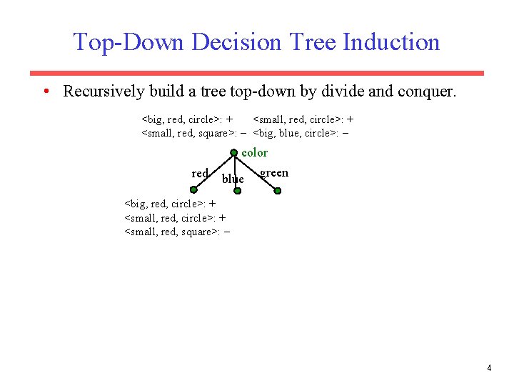
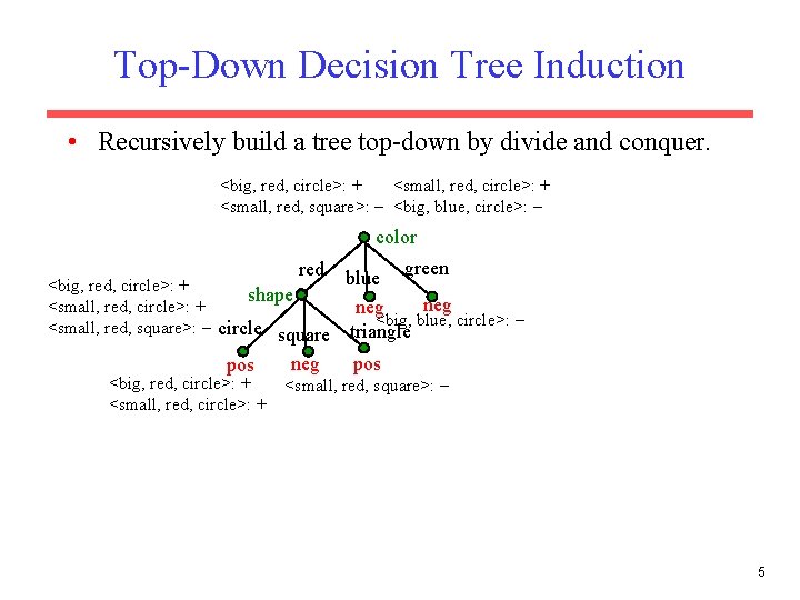
Top-Down Decision Tree Induction • Recursively build a tree top-down by divide and conquer. <big, red, circle>: + <small, red, square>: <big, blue, circle>: color red blue green <big, red, circle>: + <small, red, square>: 4

Top-Down Decision Tree Induction • Recursively build a tree top-down by divide and conquer. <big, red, circle>: + <small, red, square>: <big, blue, circle>: color green blue <big, red, circle>: + shape neg <small, red, circle>: + neg <big, blue, circle>: <small, red, square>: circle square triangle pos neg pos red <big, red, circle>: + <small, red, square>: 5

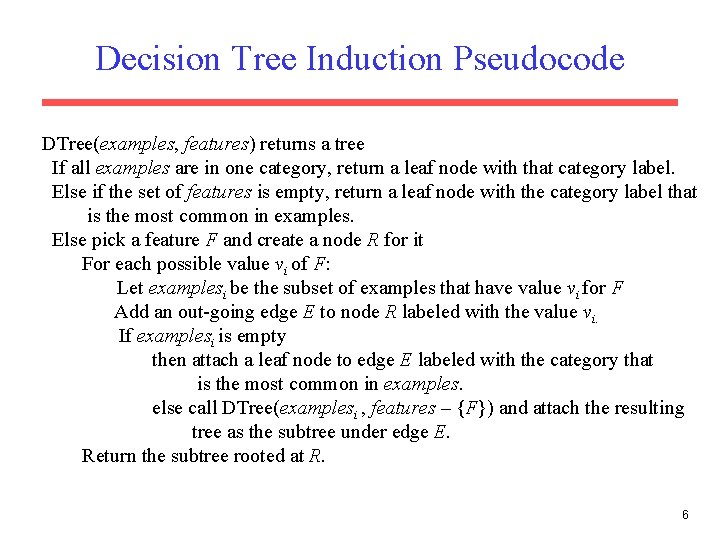
Decision Tree Induction Pseudocode DTree(examples, features) returns a tree If all examples are in one category, return a leaf node with that category label. Else if the set of features is empty, return a leaf node with the category label that is the most common in examples. Else pick a feature F and create a node R for it For each possible value vi of F: Let examplesi be the subset of examples that have value vi for F Add an out-going edge E to node R labeled with the value vi. If examplesi is empty then attach a leaf node to edge E labeled with the category that is the most common in examples. else call DTree(examplesi , features – {F}) and attach the resulting tree as the subtree under edge E. Return the subtree rooted at R. 6

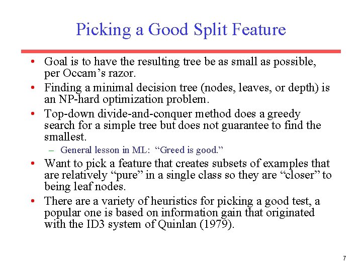
Picking a Good Split Feature • Goal is to have the resulting tree be as small as possible, per Occam’s razor. • Finding a minimal decision tree (nodes, leaves, or depth) is an NP-hard optimization problem. • Top-down divide-and-conquer method does a greedy search for a simple tree but does not guarantee to find the smallest. – General lesson in ML: “Greed is good. ” • Want to pick a feature that creates subsets of examples that are relatively “pure” in a single class so they are “closer” to being leaf nodes. • There a variety of heuristics for picking a good test, a popular one is based on information gain that originated with the ID 3 system of Quinlan (1979). 7

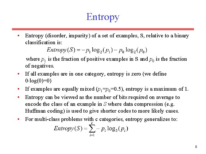
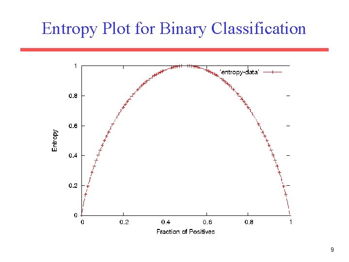
Entropy • Entropy (disorder, impurity) of a set of examples, S, relative to a binary classification is: • • where p 1 is the fraction of positive examples in S and p 0 is the fraction of negatives. If all examples are in one category, entropy is zero (we define 0 log(0)=0) If examples are equally mixed (p 1=p 0=0. 5), entropy is a maximum of 1. Entropy can be viewed as the number of bits required on average to encode the class of an example in S where data compression (e. g. Huffman coding) is used to give shorter codes to more likely cases. For multi-class problems with c categories, entropy generalizes to: 8

Entropy Plot for Binary Classification 9

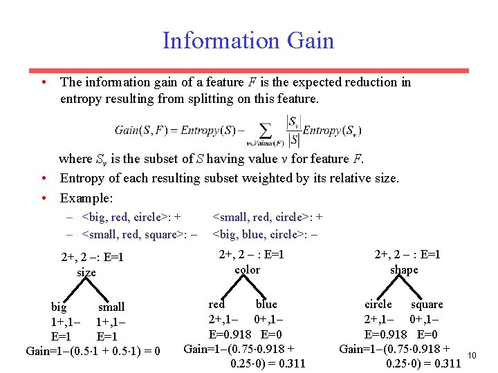
Information Gain • The information gain of a feature F is the expected reduction in entropy resulting from splitting on this feature. where Sv is the subset of S having value v for feature F. • Entropy of each resulting subset weighted by its relative size. • Example: – <big, red, circle>: + – <small, red, square>: 2+, 2 : E=1 size big small 1+, 1 E=1 Gain=1 (0. 5 1 + 0. 5 1) = 0 <small, red, circle>: + <big, blue, circle>: 2+, 2 : E=1 color red blue 2+, 1 0+, 1 E=0. 918 E=0 Gain=1 (0. 75 0. 918 + 0. 25 0) = 0. 311 2+, 2 : E=1 shape circle square 2+, 1 0+, 1 E=0. 918 E=0 Gain=1 (0. 75 0. 918 + 0. 25 0) = 0. 311 10

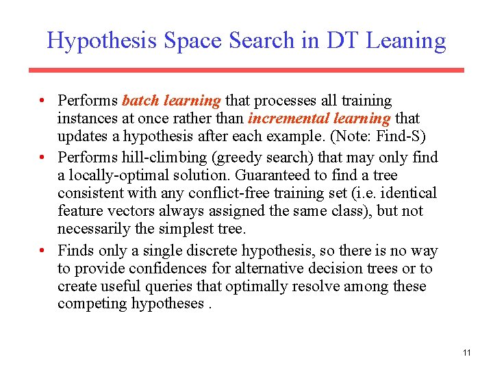
Hypothesis Space Search in DT Leaning • Performs batch learning that processes all training instances at once rather than incremental learning that updates a hypothesis after each example. (Note: Find-S) • Performs hill-climbing (greedy search) that may only find a locally-optimal solution. Guaranteed to find a tree consistent with any conflict-free training set (i. e. identical feature vectors always assigned the same class), but not necessarily the simplest tree. • Finds only a single discrete hypothesis, so there is no way to provide confidences for alternative decision trees or to create useful queries that optimally resolve among these competing hypotheses. 11

Bias in Decision-Tree Induction • Information-gain gives a bias for trees with minimal depth. • Implements a search (preference) bias instead of a language (restriction) bias. 12

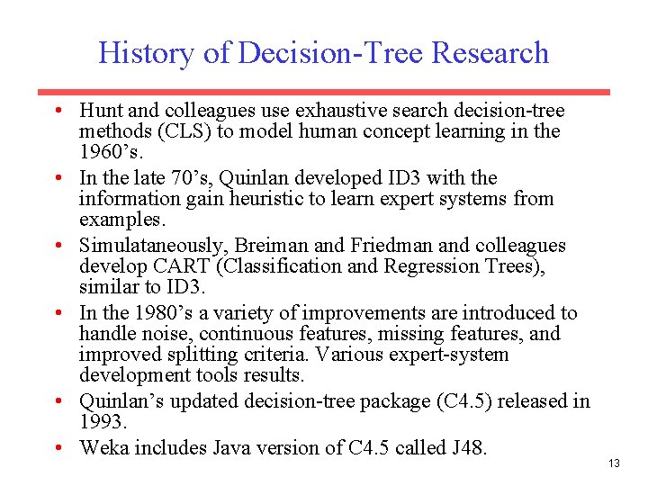
History of Decision-Tree Research • Hunt and colleagues use exhaustive search decision-tree methods (CLS) to model human concept learning in the 1960’s. • In the late 70’s, Quinlan developed ID 3 with the information gain heuristic to learn expert systems from examples. • Simulataneously, Breiman and Friedman and colleagues develop CART (Classification and Regression Trees), similar to ID 3. • In the 1980’s a variety of improvements are introduced to handle noise, continuous features, missing features, and improved splitting criteria. Various expert-system development tools results. • Quinlan’s updated decision-tree package (C 4. 5) released in 1993. • Weka includes Java version of C 4. 5 called J 48. 13

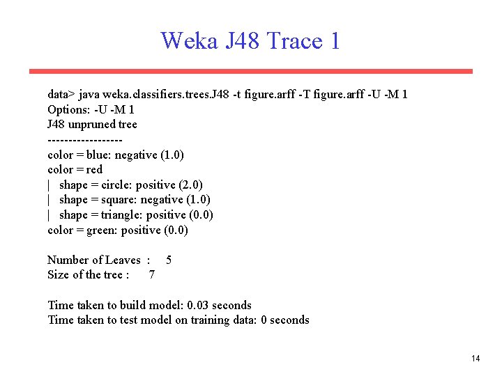
Weka J 48 Trace 1 data> java weka. classifiers. trees. J 48 -t figure. arff -T figure. arff -U -M 1 Options: -U -M 1 J 48 unpruned tree ---------color = blue: negative (1. 0) color = red | shape = circle: positive (2. 0) | shape = square: negative (1. 0) | shape = triangle: positive (0. 0) color = green: positive (0. 0) Number of Leaves : 5 Size of the tree : 7 Time taken to build model: 0. 03 seconds Time taken to test model on training data: 0 seconds 14

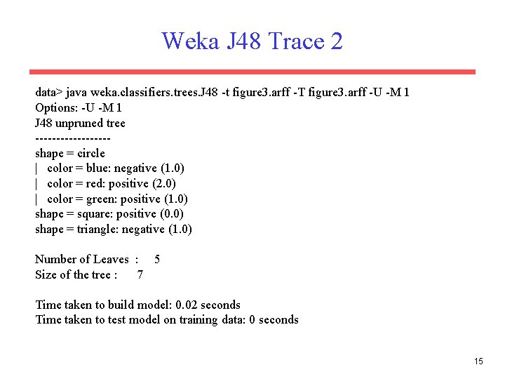
Weka J 48 Trace 2 data> java weka. classifiers. trees. J 48 -t figure 3. arff -T figure 3. arff -U -M 1 Options: -U -M 1 J 48 unpruned tree ---------shape = circle | color = blue: negative (1. 0) | color = red: positive (2. 0) | color = green: positive (1. 0) shape = square: positive (0. 0) shape = triangle: negative (1. 0) Number of Leaves : 5 Size of the tree : 7 Time taken to build model: 0. 02 seconds Time taken to test model on training data: 0 seconds 15

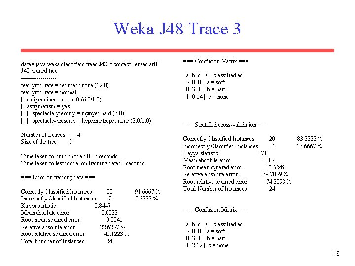
Weka J 48 Trace 3 data> java weka. classifiers. trees. J 48 -t contact-lenses. arff J 48 pruned tree ---------tear-prod-rate = reduced: none (12. 0) tear-prod-rate = normal | astigmatism = no: soft (6. 0/1. 0) | astigmatism = yes | | spectacle-prescrip = myope: hard (3. 0) | | spectacle-prescrip = hypermetrope: none (3. 0/1. 0) Number of Leaves : 4 Size of the tree : 7 Time taken to build model: 0. 03 seconds Time taken to test model on training data: 0 seconds === Error on training data === Correctly Classified Instances 22 91. 6667 % Incorrectly Classified Instances 2 8. 3333 % Kappa statistic 0. 8447 Mean absolute error 0. 0833 Root mean squared error 0. 2041 Relative absolute error 22. 6257 % Root relative squared error 48. 1223 % Total Number of Instances 24 === Confusion Matrix === a 5 0 1 b c <-- classified as 0 0 | a = soft 3 1 | b = hard 0 14 | c = none === Stratified cross-validation === Correctly Classified Instances 20 83. 3333 % Incorrectly Classified Instances 4 16. 6667 % Kappa statistic 0. 71 Mean absolute error 0. 15 Root mean squared error 0. 3249 Relative absolute error 39. 7059 % Root relative squared error 74. 3898 % Total Number of Instances 24 === Confusion Matrix === a 5 0 1 b c <-- classified as 0 0 | a = soft 3 1 | b = hard 2 12 | c = none 16

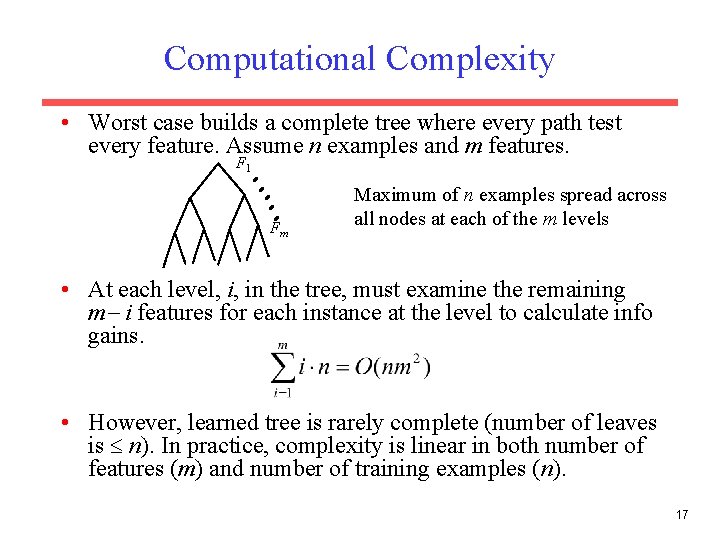
Computational Complexity • Worst case builds a complete tree where every path test every feature. Assume n examples and m features. F 1 Fm Maximum of n examples spread across all nodes at each of the m levels • At each level, i, in the tree, must examine the remaining m i features for each instance at the level to calculate info gains. • However, learned tree is rarely complete (number of leaves is n). In practice, complexity is linear in both number of features (m) and number of training examples (n). 17

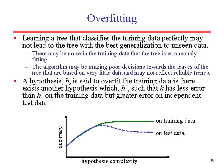
Overfitting • Learning a tree that classifies the training data perfectly may not lead to the tree with the best generalization to unseen data. – There may be noise in the training data that the tree is erroneously fitting. – The algorithm may be making poor decisions towards the leaves of the tree that are based on very little data and may not reflect reliable trends. • A hypothesis, h, is said to overfit the training data is there exists another hypothesis which, h´, such that h has less error than h´ on the training data but greater error on independent test data. accuracy on training data on test data hypothesis complexity 18

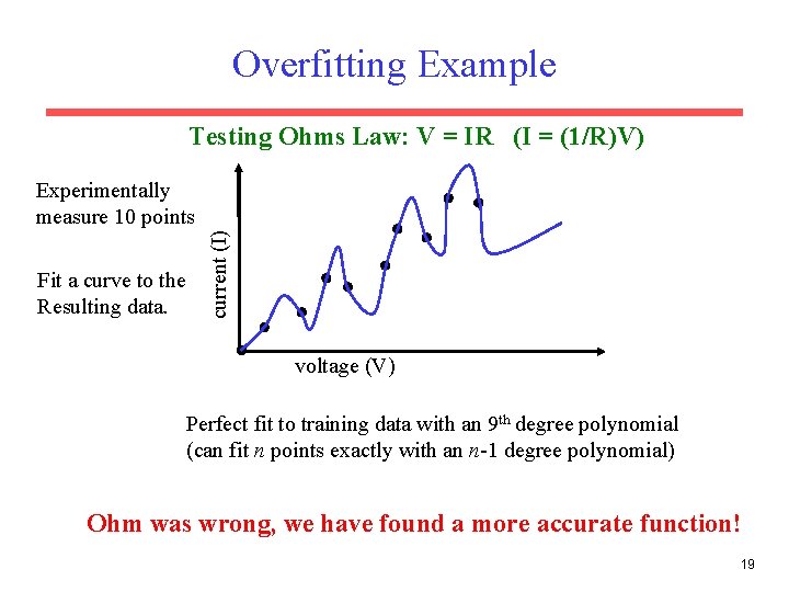
Overfitting Example Testing Ohms Law: V = IR (I = (1/R)V) Fit a curve to the Resulting data. current (I) Experimentally measure 10 points voltage (V) Perfect fit to training data with an 9 th degree polynomial (can fit n points exactly with an n-1 degree polynomial) Ohm was wrong, we have found a more accurate function! 19

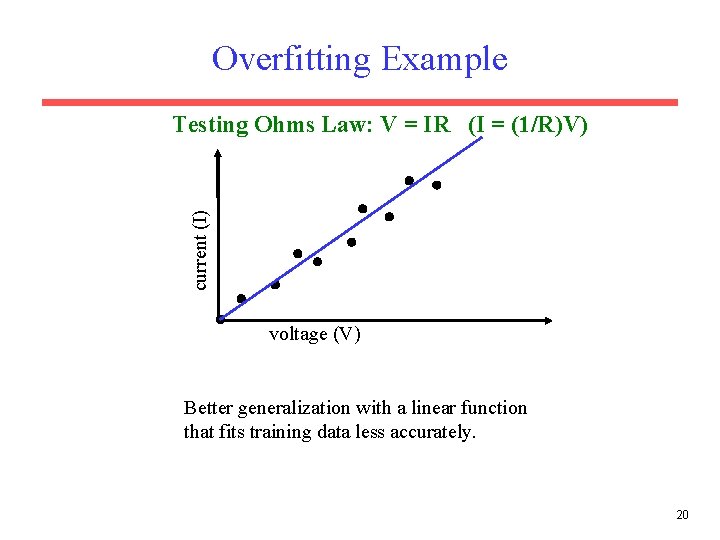
Overfitting Example current (I) Testing Ohms Law: V = IR (I = (1/R)V) voltage (V) Better generalization with a linear function that fits training data less accurately. 20

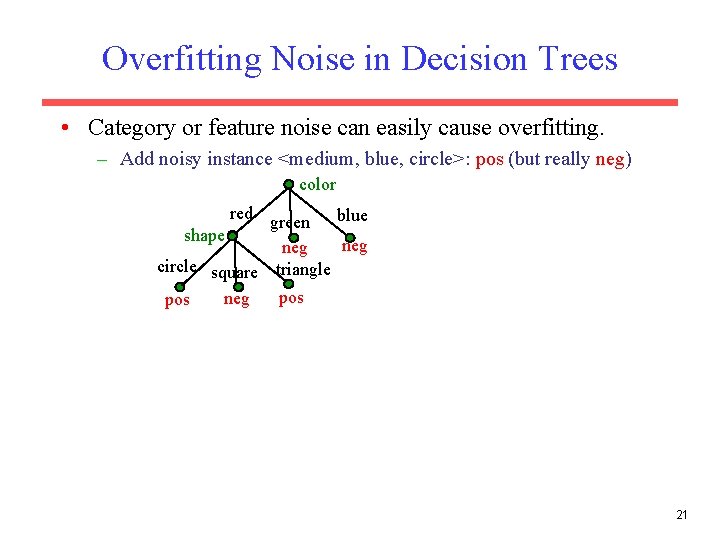
Overfitting Noise in Decision Trees • Category or feature noise can easily cause overfitting. – Add noisy instance <medium, blue, circle>: pos (but really neg) color red green blue shape neg circle square triangle pos neg pos 21

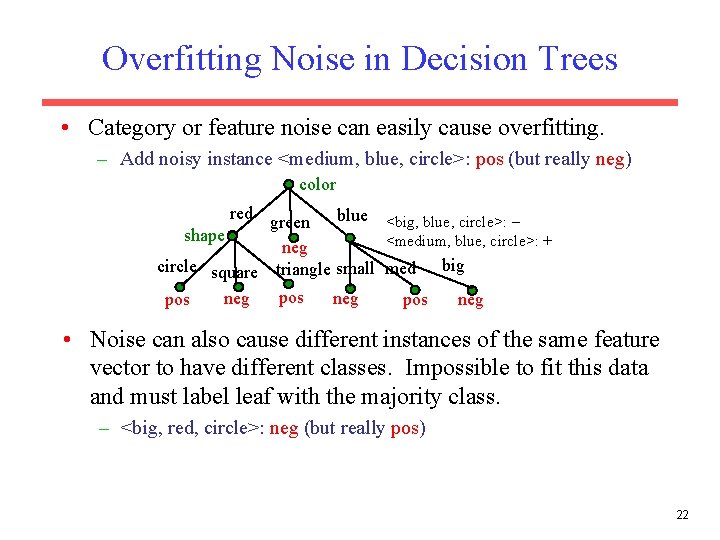
Overfitting Noise in Decision Trees • Category or feature noise can easily cause overfitting. – Add noisy instance <medium, blue, circle>: pos (but really neg) color red green blue <big, blue, circle>: shape <medium, blue, circle>: + neg circle square triangle small med big pos neg • Noise can also cause different instances of the same feature vector to have different classes. Impossible to fit this data and must label leaf with the majority class. – <big, red, circle>: neg (but really pos) 22

Overfitting Prevention (Pruning) Methods • Two basic approaches for decision trees – Prepruning: Stop growing tree as some point during top-down construction when there is no longer sufficient data to make reliable decisions. : Where to stop? – Postpruning: Grow the full tree, then remove subtrees that do not have sufficient evidence. • Label leaf resulting from pruning with the majority class of the remaining data, or a class probability distribution. • Method for determining which subtrees to prune: – Cross-validation: Reserve some training data as a hold-out set (validation set, tuning set) to evaluate utility of subtrees. – Statistical test: Use a statistical (chi-square) test on the training data to estimate whether expanding a particular node is likely to produce an improvement beyond the training set. – Minimum description length (MDL): . Use measure of complexity for encoding the training examples and the decision tree, halting growth of the tree when the encoding size is minimized. 23

Reduced Error Pruning • A post-pruning, cross-validation approach. Partition training data in “grow(2/3)” and “validation(1/3)” sets. Build a complete tree from the “grow” data. Until accuracy on validation set decreases do: For each non-leaf node, n, in the tree do: Temporarily prune the subtree below n and replace it with a leaf labeled with the current majority class at that node. Measure and record the accuracy of the pruned tree on the validation set. Permanently prune the node that results in the greatest increase in accuracy on the validation set. 24

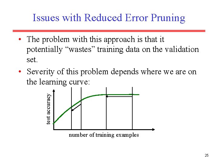
Issues with Reduced Error Pruning test accuracy • The problem with this approach is that it potentially “wastes” training data on the validation set. • Severity of this problem depends where we are on the learning curve: number of training examples 25

Cross-Validating without Losing Training Data • If the algorithm is modified to grow trees breadthfirst rather than depth-first, we can stop growing after reaching any specified tree complexity. • First, run several trials of reduced error-pruning using different random splits of grow and validation sets. • Record the complexity of the pruned tree learned in each trial. Let C be the average pruned-tree complexity. • Grow a final tree breadth-first from all the training data but stop when the complexity reaches C. • Similar cross-validation approach can be used to set arbitrary algorithm parameters in general. 26

Rule Post-Pruning • Procedure – Construct DT from training data set allowing overfitting to occur – Convert the DT to rules in which each path from root to leaf node becomes a rule – Prune each rule by removing any preconditions that result in improving its estimated accuracy. – Sort the pruned rules by their estimated accuracy and consider them in this sequence when classifying subsequent instances. 27

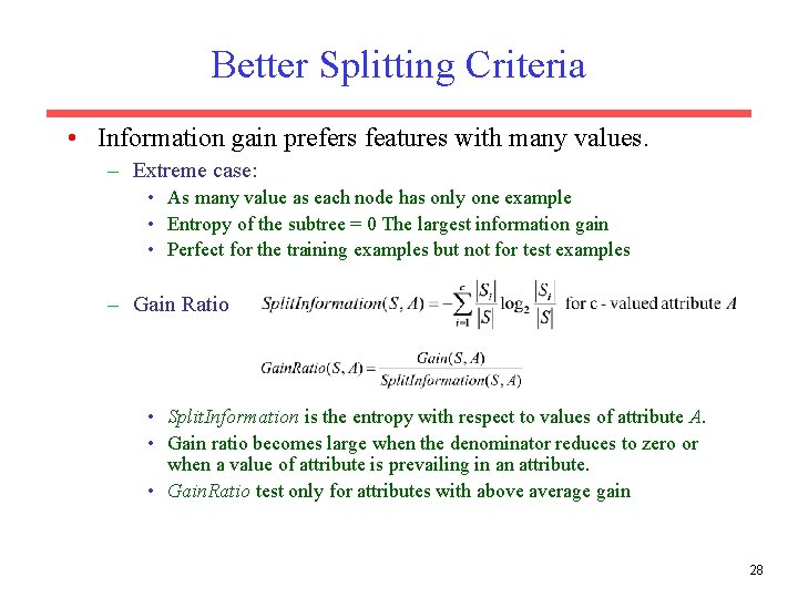
Better Splitting Criteria • Information gain prefers features with many values. – Extreme case: • As many value as each node has only one example • Entropy of the subtree = 0 The largest information gain • Perfect for the training examples but not for test examples – Gain Ratio • Split. Information is the entropy with respect to values of attribute A. • Gain ratio becomes large when the denominator reduces to zero or when a value of attribute is prevailing in an attribute. • Gain. Ratio test only for attributes with above average gain 28

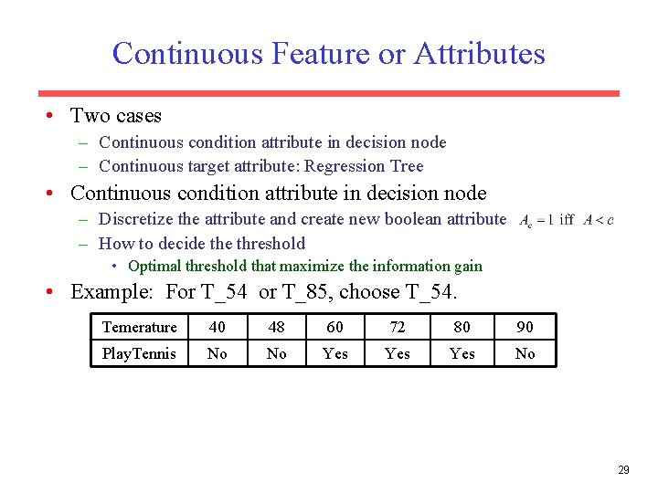
Continuous Feature or Attributes • Two cases – Continuous condition attribute in decision node – Continuous target attribute: Regression Tree • Continuous condition attribute in decision node – Discretize the attribute and create new boolean attribute – How to decide threshold • Optimal threshold that maximize the information gain • Example: For T_54 or T_85, choose T_54. Temerature 40 48 60 72 80 90 Play. Tennis No No Yes Yes No 29

Regression Trees: 30

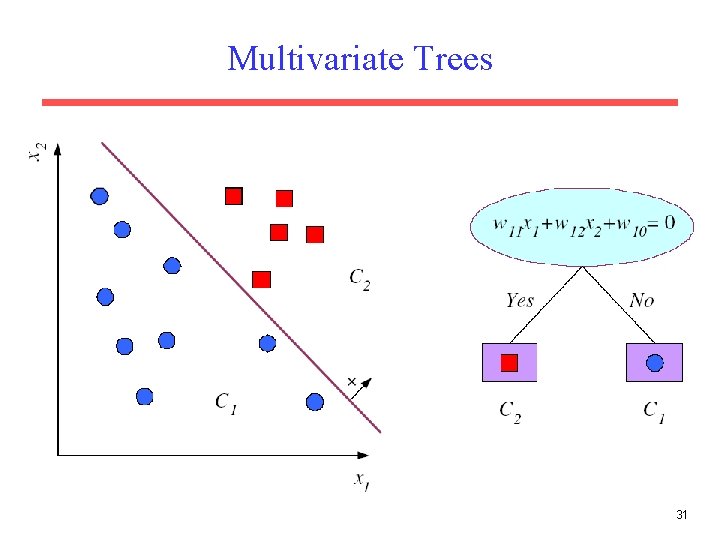
Multivariate Trees 31

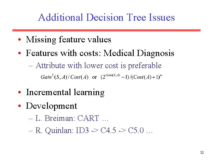
Additional Decision Tree Issues • Missing feature values • Features with costs: Medical Diagnosis – Attribute with lower cost is preferable • Incremental learning • Development – L. Breiman: CART … – R. Quinlan: ID 3 -> C 4. 5 -> C 5. 0 … 32