Machine Learning Data visualization and dimensionality reduction Eric

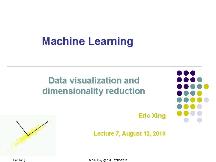
Machine Learning Data visualization and dimensionality reduction Eric Xing Lecture 7, August 13, 2010 Eric Xing © Eric Xing @ CMU, 2006 -2010

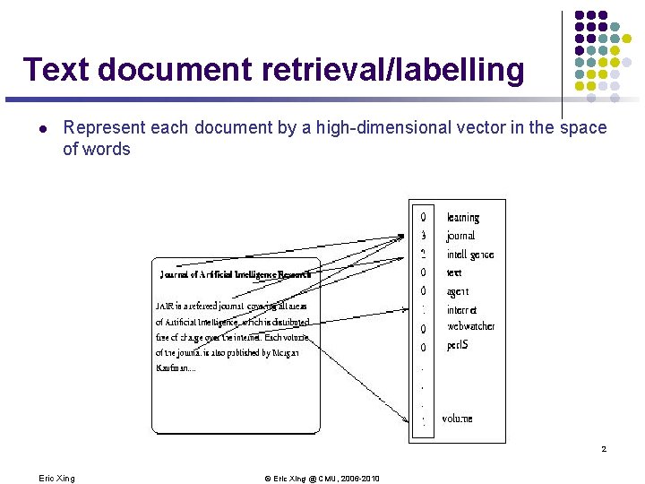
Text document retrieval/labelling l Represent each document by a high-dimensional vector in the space of words 2 Eric Xing © Eric Xing @ CMU, 2006 -2010

Image retrieval/labelling 3 Eric Xing © Eric Xing @ CMU, 2006 -2010

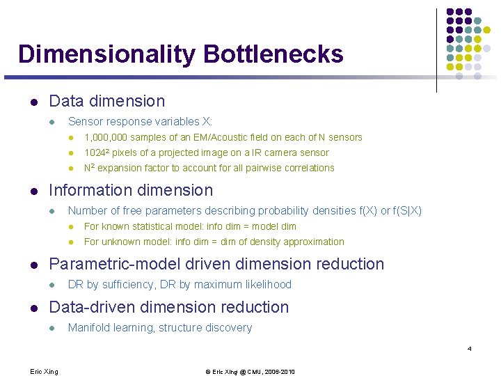
Dimensionality Bottlenecks l Data dimension l l 1, 000 samples of an EM/Acoustic field on each of N sensors l 10242 pixels of a projected image on a IR camera sensor l N 2 expansion factor to account for all pairwise correlations Number of free parameters describing probability densities f(X) or f(S|X) l For known statistical model: info dim = model dim l For unknown model: info dim = dim of density approximation Parametric-model driven dimension reduction l l l Information dimension l l Sensor response variables X: DR by sufficiency, DR by maximum likelihood Data-driven dimension reduction l Manifold learning, structure discovery 4 Eric Xing © Eric Xing @ CMU, 2006 -2010

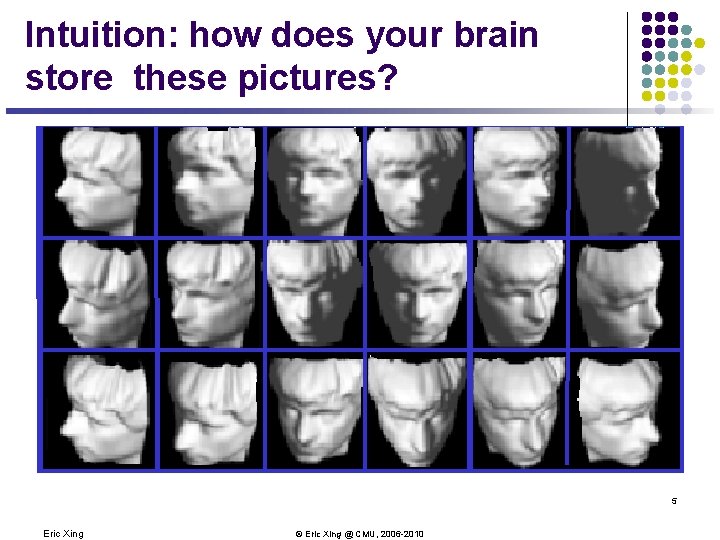
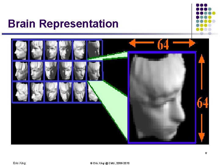
Intuition: how does your brain store these pictures? 5 Eric Xing © Eric Xing @ CMU, 2006 -2010

Brain Representation 6 Eric Xing © Eric Xing @ CMU, 2006 -2010

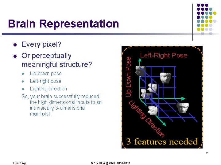
Brain Representation l Every pixel? l Or perceptually meaningful structure? l Up-down pose l Left-right pose l Lighting direction So, your brain successfully reduced the high-dimensional inputs to an intrinsically 3 -dimensional manifold! 7 Eric Xing © Eric Xing @ CMU, 2006 -2010

Two Geometries to Consider (Metric) data geometry (Non-metric) information geometry Manifold Embedding Domain are i. i. d. samples from 8 Eric Xing © Eric Xing @ CMU, 2006 -2010

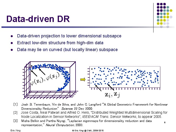
Data-driven DR l Data-driven projection to lower dimensional subsapce l Extract low-dim structure from high-dim data l Data may lie on curved (but locally linear) subspace [1] [2] [3] Eric Xing Josh. B. Tenenbaum, Vin de Silva, and John C. Langford “A Global Geometric Framework for Nonlinear Dimensionality Reduction” Science, 22 Dec 2000. Jose Costa, Neal Patwari and Alfred O. Hero, “Distributed Weighted Multidimensional Scaling for Node Localization in Sensor Networks”, IEEE/ACM Trans. Sensor Networks, to appear 2005. Misha Belkin and Partha Niyogi, “Laplacian eigenmaps for dimensionality reduction and data 9 representation, ” Neural Computation, 2003. © Eric Xing @ CMU, 2006 -2010

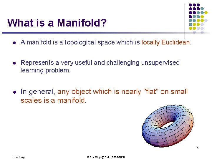
What is a Manifold? l A manifold is a topological space which is locally Euclidean. l Represents a very useful and challenging unsupervised learning problem. l In general, any object which is nearly "flat" on small scales is a manifold. 10 Eric Xing © Eric Xing @ CMU, 2006 -2010

Manifold Learning l Discover low dimensional structures (smooth manifold) for data in high dimension. l Linear Approaches l l Principal component analysis. l Multi dimensional scaling. Non Linear Approaches l Local Linear Embedding l ISOMAP l Laplacian Eigenmap. 11 Eric Xing © Eric Xing @ CMU, 2006 -2010

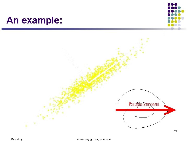
Principal component analysis l Areas of variance in data are where items can be best discriminated and key underlying phenomena observed l If two items or dimensions are highly correlated or dependent l They are likely to represent highly related phenomena l We want to combine related variables, and focus on uncorrelated or independent ones, especially those along which the observations have high variance l We look for the phenomena underlying the observed covariance/codependence in a set of variables l These phenomena are called “factors” or “principal components” or “independent components, ” depending on the methods used l Factor analysis: based on variance/correlation l Independent Component Analysis: based on independence 12 Eric Xing © Eric Xing @ CMU, 2006 -2010

An example: 13 Eric Xing © Eric Xing @ CMU, 2006 -2010

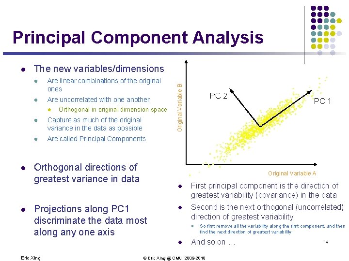
Principal Component Analysis The new variables/dimensions l Are linear combinations of the original ones l Are uncorrelated with one another l l l Orthogonal in original dimension space l Capture as much of the original variance in the data as possible l Are called Principal Components Orthogonal directions of greatest variance in data Original Variable B l PC 1 Original Variable A Projections along PC 1 discriminate the data most along any one axis l First principal component is the direction of greatest variability (covariance) in the data l Second is the next orthogonal (uncorrelated) direction of greatest variability l l Eric Xing PC 2 So first remove all the variability along the first component, and then find the next direction of greatest variability And so on … © Eric Xing @ CMU, 2006 -2010 14

Computing the Components l Projection of vector x onto an axis (dimension) u is u. Tx l Direction of greatest variability is that in which the average square of the projection is greatest: Maximize u. TXXTu s. t u Tu = 1 Construct Langrangian u. TXXTu – λu. Tu Vector of partial derivatives set to zero xx. Tu – λu = (xx. T – λI) u = 0 As u ≠ 0 then u must be an eigenvector of XXT with eigenvalue λ l l Eric Xing l is the principal eigenvalue of the correlation matrix C= XXT The eigenvalue denotes the amount of variability captured along that dimension © Eric Xing @ CMU, 2006 -2010 15

Computing the Components l Similarly for the next axis, etc. l So, the new axes are the eigenvectors of the matrix of correlations of the original variables, which captures the similarities of the original variables based on how data samples project to them l Geometrically: centering followed by rotation l Eric Xing Linear transformation © Eric Xing @ CMU, 2006 -2010 16

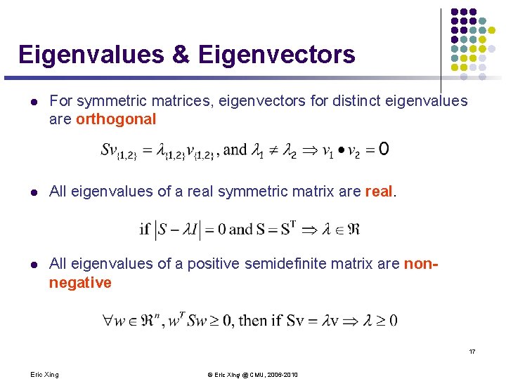
Eigenvalues & Eigenvectors l For symmetric matrices, eigenvectors for distinct eigenvalues are orthogonal l All eigenvalues of a real symmetric matrix are real. l All eigenvalues of a positive semidefinite matrix are nonnegative 17 Eric Xing © Eric Xing @ CMU, 2006 -2010

Eigen/diagonal Decomposition l l Let be a square matrix with m linearly independent eigenvectors (a “non-defective” matrix) Theorem: Exists an eigen decomposition diagonal Unique for distinct eigenvalues (cf. matrix diagonalization theorem) l Columns of U are eigenvectors of S l Diagonal elements of are eigenvalues of 18 Eric Xing © Eric Xing @ CMU, 2006 -2010

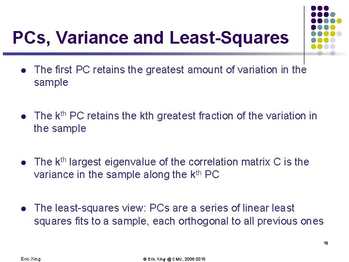
PCs, Variance and Least-Squares l The first PC retains the greatest amount of variation in the sample l The kth PC retains the kth greatest fraction of the variation in the sample l The kth largest eigenvalue of the correlation matrix C is the variance in the sample along the kth PC l The least-squares view: PCs are a series of linear least squares fits to a sample, each orthogonal to all previous ones 19 Eric Xing © Eric Xing @ CMU, 2006 -2010

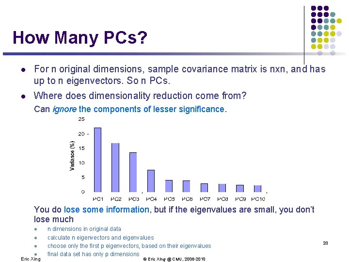
How Many PCs? l For n original dimensions, sample covariance matrix is nxn, and has up to n eigenvectors. So n PCs. l Where does dimensionality reduction come from? Can ignore the components of lesser significance. You do lose some information, but if the eigenvalues are small, you don’t lose much l l Eric Xing n dimensions in original data calculate n eigenvectors and eigenvalues choose only the first p eigenvectors, based on their eigenvalues final data set has only p dimensions © Eric Xing @ CMU, 2006 -2010 20

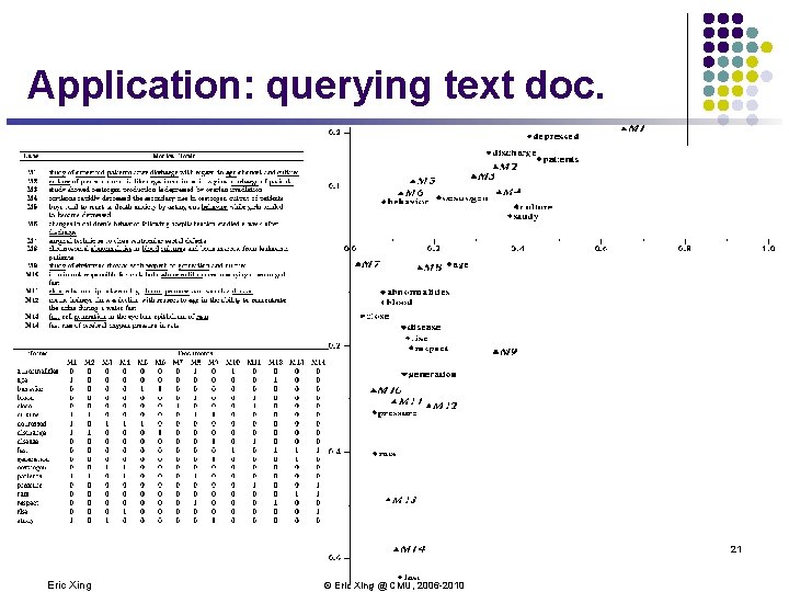
Application: querying text doc. 21 Eric Xing © Eric Xing @ CMU, 2006 -2010

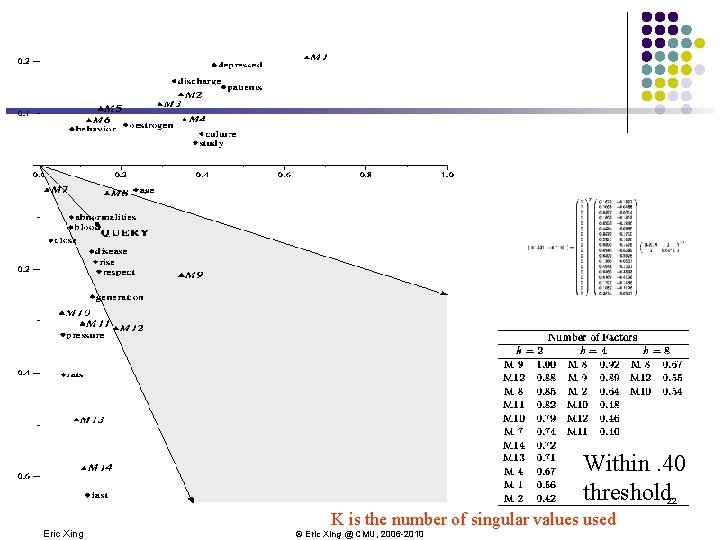
Within. 40 threshold 22 Eric Xing K is the number of singular values used © Eric Xing @ CMU, 2006 -2010

Summary: l l l Principle l Linear projection method to reduce the number of parameters l Transfer a set of correlated variables into a new set of uncorrelated variables l Map the data into a space of lower dimensionality l Form of unsupervised learning Properties l It can be viewed as a rotation of the existing axes to new positions in the space defined by original variables l New axes are orthogonal and represent the directions with maximum variability Application: In many settings in pattern recognition and retrieval, we have a feature-object matrix. l For text, the terms are features and the docs are objects. l Could be opinions and users … l This matrix may be redundant in dimensionality. l Can work with low-rank approximation. l If entries are missing (e. g. , users’ opinions), can recover if dimensionality is low. Eric Xing © Eric Xing @ CMU, 2006 -2010 23

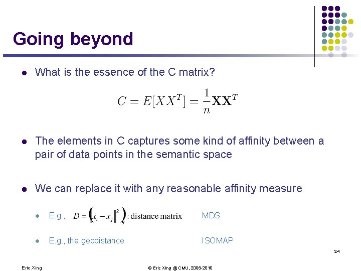
Going beyond l What is the essence of the C matrix? l The elements in C captures some kind of affinity between a pair of data points in the semantic space l We can replace it with any reasonable affinity measure l E. g. , MDS l E. g. , the geodistance ISOMAP 24 Eric Xing © Eric Xing @ CMU, 2006 -2010

Nonlinear DR – Isomap [Josh. Tenenbaum, Vin de Silva, John langford 2000] l Constructing neighbourhood graph G l For each pair of points in G, Computing shortest path distances ---- geodesic distances. l l l Use Dijkstra's or Floyd's algorithm Apply kernel PCA for C given by the centred matrix of squared geodesic distances. Project test points onto principal components as in kernel PCA. 25 Eric Xing © Eric Xing @ CMU, 2006 -2010

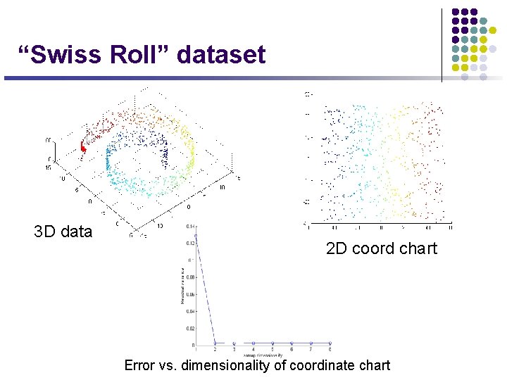
“Swiss Roll” dataset 3 D data 2 D coord chart Error vs. dimensionality of coordinate chart

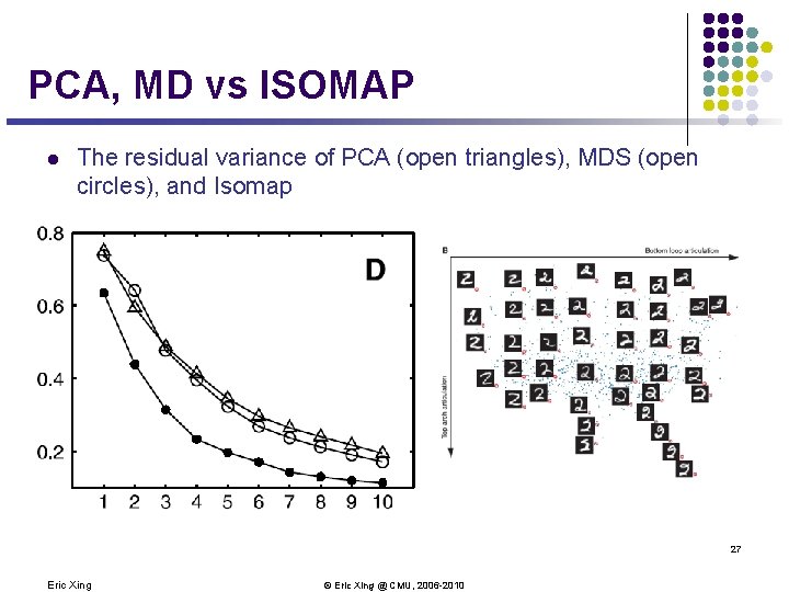
PCA, MD vs ISOMAP l The residual variance of PCA (open triangles), MDS (open circles), and Isomap 27 Eric Xing © Eric Xing @ CMU, 2006 -2010

ISOMAP algorithm Pros/Cons Advantages: l Nonlinear l Globally optimal l Guarantee asymptotically to recover the true dimensionality Drawback: l May not be stable, dependent on topology of data l As N increases, pair wise distances provide better approximations to geodesics, but cost more computation 28 Eric Xing © Eric Xing @ CMU, 2006 -2010

Local Linear Embedding (a. k. a LLE) l LLE is based on simple geometric intuitions. l Suppose the data consist of N real-valued vectors Xi, each of dimensionality D. l Each data point and its neighbors expected to lie on or close to a locally linear patch of the manifold. 29 Eric Xing © Eric Xing @ CMU, 2006 -2010

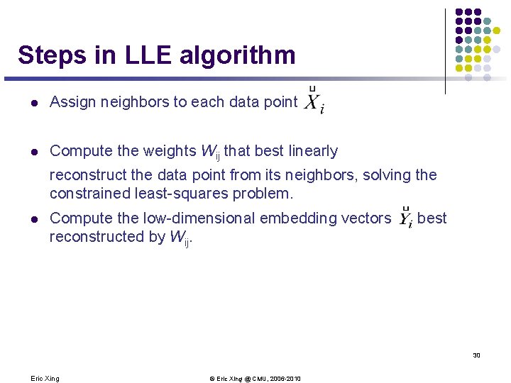
Steps in LLE algorithm l Assign neighbors to each data point l Compute the weights Wij that best linearly reconstruct the data point from its neighbors, solving the constrained least-squares problem. l Compute the low-dimensional embedding vectors reconstructed by Wij. best 30 Eric Xing © Eric Xing @ CMU, 2006 -2010

Fit locally, Think Globally From Nonlinear Dimensionality Reduction by Locally Linear Embedding Sam T. Roweis and Lawrence K. Saul 31 Eric Xing © Eric Xing @ CMU, 2006 -2010

Super-Resolution Through Neighbor Embedding [Yeung et al CVPR 2004] Training Xsi Training Ysi ? Testing Xt 32 Eric Xing Testing Yt © Eric Xing @ CMU, 2006 -2010

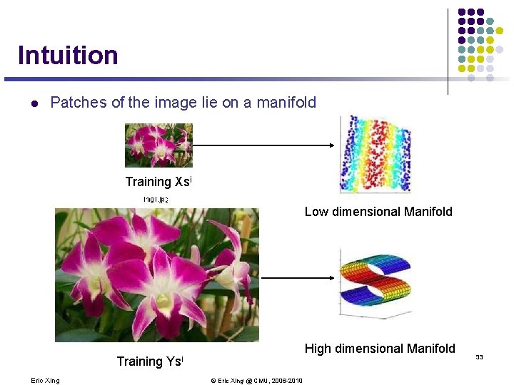
Intuition l Patches of the image lie on a manifold Training Xsi Low dimensional Manifold Training Eric Xing High dimensional Manifold Ysi © Eric Xing @ CMU, 2006 -2010 33

Algorithm 1. Get feature vectors for each low resolution training patch. 2. For each test patch feature vector find K nearest neighboring feature vectors of training patches. 3. Find optimum weights to express each test patch vector as a weighted sum of its K nearest neighbor vectors. 4. Use these weights for reconstruction of that test patch in high resolution. 34 Eric Xing © Eric Xing @ CMU, 2006 -2010

Results Training Xsi Training Ysi Testing Xt 35 Eric Xing © Eric Xing @ CMU, 2006 -2010 Testing Yt

Summary: l l Principle l Linear and nonlinear projection method to reduce the number of parameters l Transfer a set of correlated variables into a new set of uncorrelated variables l Map the data into a space of lower dimensionality l Form of unsupervised learning Applications l PCA and Latent semantic indexing for text mining l Isomap and Nonparametric Models of Image Deformation l LLE and Isomap Analysis of Spectra and Colour Images l Image Spaces and Video Trajectories: Using Isomap to Explore Video Sequences l Mining the structural knowledge of high-dimensional medical data using isomap Isomap Webpage: http: //isomap. stanford. edu/ 36 Eric Xing © Eric Xing @ CMU, 2006 -2010