Machine Learning Data Mining Part 1 The Basics
Machine Learning & Data Mining Part 1: The Basics Jaime Carbonell (with contributions from Tom Mitchell, Sebastian Thrun and Yiming Yang) Carnegie Mellon University jgc@cs. cmu. edu December, 2008 © 2008, Jaime G Carbonell
Some Definitions (KBS vs ML) o o o Knowledge-Based Systems n Rules, procedures, semantic nets, Horn clauses n Inference: matching, inheritance, resolution n Acquisition: manually from human experts Machine Learning n Data: tables, relations, attribute lists, … n Inference: rules, trees, decision functions, … n Acquisition: automated from data Data Mining n Machine learning applied to large real problems n May be augmented with KBS December, 2008 © 2008, Jaime G. Carbonell 2
Ingredients for Machine Learning o o o “Historical” data (e. g. DB tables) n E. g. products (features, marketing, support, …) n E. g. competition (products, pricing, customers) n E. g. customers (demographics, purchases, …) Objective function (to be predicted or optimized) n E. g. maximize revenue per customer n E. g. minimize manufacturing defects Scalable machine learning method(s) n E. g. decision-tree induction, logistic regression n E. g. “active” learning, clustering December, 2008 © 2008, Jaime G. Carbonell 3
Sample ML/DM Applications I o o Credit Scoring n Training: past applicant profiles, how much credit given, payback or default n Input: applicant profile (income, debts, …) n Objective: credit-score + max amount Fraud Detection (e. g. credit-card transactions) n Training: past known legitimate & fraudulent transactions n Input: proposed transaction (loc, cust, $$, …) n Objective: approve/block decision December, 2008 © 2008, Jaime G. Carbonell 4
Sample ML/DM Applications II o o Demographic Segmentation n Training: past customer profiles (age, gender, education, income, …) + product preferences n Input: new product description (features) n Objective: predict market segment affinity Marketing/Advertisement Effectiveness n Training: past advertisement campaigns, demographic targets, product categories n Input: proposed advertisement campaign n Objective: project effectiveness (sales increase modulated by marketing cost) December, 2008 © 2008, Jaime G. Carbonell 5
Sample ML/DM Applications III o o Product (or Part) Reliability n Training: past products/parts + specs at manufacturing + customer usage + maint rec n Input: new part + expected usage n Objective: mean-time-to-failure (replacement) Manufacturing Tolerances n Training: past product/part manufacturing process, tolerances, inspections, … n Input: new part + expected usage n Objective: optimal manufacturing precision (minimize costs of failure + manufacture) December, 2008 © 2008, Jaime G. Carbonell 6
Sample ML/DM Applications IV o o Mechanical Diagnosis n Training: past observed symptoms at (or prior to) breakdown + underlying cause n Input: current symptoms n Objective: predict cause of failure Mechanical Repair n Training: cause of failure + product usage + repair (or PM) effectiveness n Input: new failure cause + product usage n Objective: recommended repair (or preventive maintenance operation) December, 2008 © 2008, Jaime G. Carbonell 7
Sample ML/DM Applications V o o Billeting (job assignments) n Training: employee profiles, position profiles, employee performance in assigned position n Input: new employee or new position profile n Objective: predict performance in position Text Mining & Routing (e. g. customer centers) n Training: electronic problem reports, customer requests + who should handle them n Input: new incoming texts n Objective: Assign category + route or reply December, 2008 © 2008, Jaime G. Carbonell 8
Preparing Historical Data o o o Extract a DB table with all the needed information n Select, join, project, aggregate, … n Filter out rows with significant missing data Determine predictor attributes (columns) n Ask domain expert for relevant attributes, or n Start with all attributes and automatically subselect most predictive ones (feature selection) Determine to-be-predicted attribute (column) n Objective of the DM (number, decision, …) December, 2008 © 2008, Jaime G. Carbonell 9
![Sample DB Table [predictor attributes] [objective] Tot Num Max Num Acct. Income Job Delinq Sample DB Table [predictor attributes] [objective] Tot Num Max Num Acct. Income Job Delinq](http://slidetodoc.com/presentation_image_h2/032abf1a98a880dfead4cec596820e5e/image-10.jpg)
Sample DB Table [predictor attributes] [objective] Tot Num Max Num Acct. Income Job Delinq Owns Credit Good numb. in K/yr Now? accts cycles home? years cust. ? -------------------------------------1001 85 Y 1 1 N 2 Y 1002 60 Y 3 2 Y 5 N 1003 ? N 0 0 N 2 N 1004 95 Y 1 2 N 9 Y 1005 110 Y 1 6 Y 3 Y 1006 29 Y 2 1 Y 1 N 1007 88 Y 6 4 Y 8 N 1008 80 Y 0 Y 1009 31 Y 1 1 N 1 Y 1011 ? Y ? 0 ? 7 Y 1012 75 ? 2 4 N 2 N 1013 20 N 1 1 N 3 N 1014 65 Y 1 3 Y 1015 65 N 1 2 N 8 Y 1016 20 N 0 N 1017 75 Y 1 3 N 2 N 1018 40 N 0 0 Y 1 Y December, 2008 © 2008, Jaime G. Carbonell 10
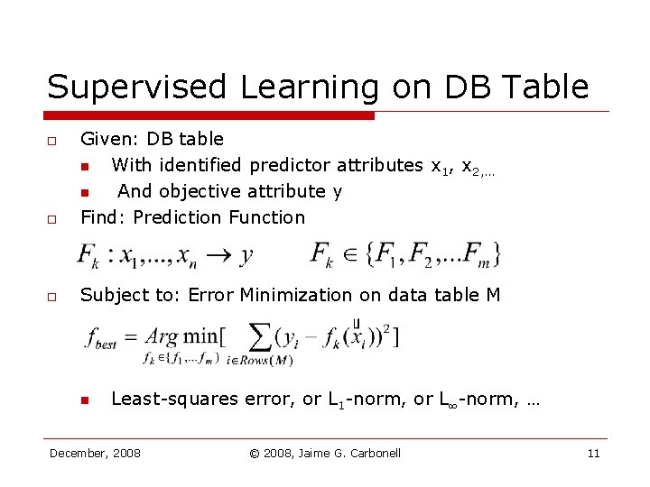
Supervised Learning on DB Table o Given: DB table n With identified predictor attributes x 1, x 2, … n And objective attribute y Find: Prediction Function o Subject to: Error Minimization on data table M o n Least-squares error, or L 1 -norm, or L -norm, … December, 2008 © 2008, Jaime G. Carbonell 11
Popular Predictor Functions o o o o Linear Discriminators (next slides) k-Nearest-Neighbors (lecture #2) Decision Trees (lecture #5) Linear & Logistic Regression (lecture #4) Probabilistic Methods (Lecture #3) Neural Networks n 2 -layer Logistic Regression n Multi-layer Difficult to scale up Classification Rule Induction (in a few slides) December, 2008 © 2008, Jaime G. Carbonell 12
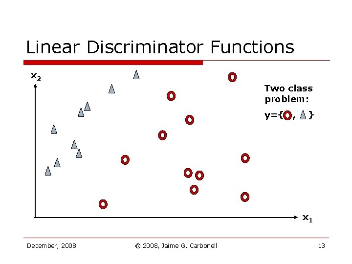
Linear Discriminator Functions x 2 Two class problem: y={ , } x 1 December, 2008 © 2008, Jaime G. Carbonell 13
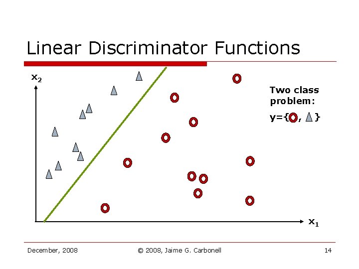
Linear Discriminator Functions x 2 Two class problem: y={ , } x 1 December, 2008 © 2008, Jaime G. Carbonell 14
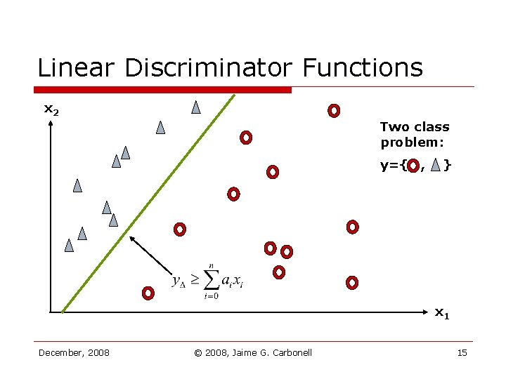
Linear Discriminator Functions x 2 Two class problem: y={ , } x 1 December, 2008 © 2008, Jaime G. Carbonell 15

Linear Discriminator Functions x 2 Two class problem: new y={ , } x 1 December, 2008 © 2008, Jaime G. Carbonell 16
Issues with Linear Discriminators o o o What is the “best” placement of the discriminator? n Maximize the margin n In general Support Vector Machines What if there are k classes (K > 2)? n Must learn k different discriminators n Each discriminates ki vs kj i (all other classes) What if it classes are not linearly separable? n Minimal error (L 1 or L 2) placement (regression) n Give up on linear discriminators ( other fk’s) December, 2008 © 2008, Jaime G. Carbonell 17
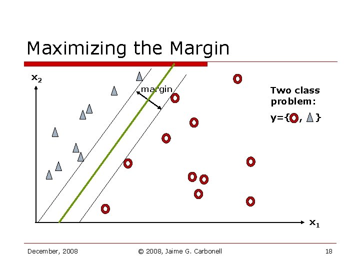
Maximizing the Margin x 2 margin Two class problem: y={ , } x 1 December, 2008 © 2008, Jaime G. Carbonell 18

Nearly-Separable Classes x 2 Two class problem: y={ , } x 1 December, 2008 © 2008, Jaime G. Carbonell 19
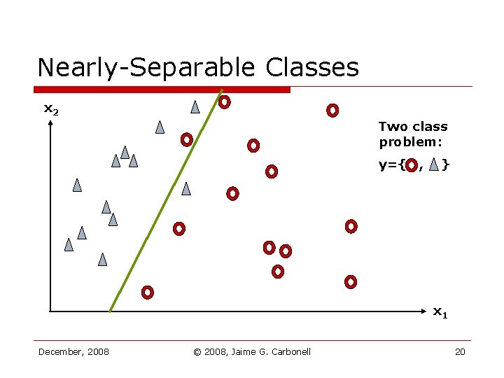
Nearly-Separable Classes x 2 Two class problem: y={ , } x 1 December, 2008 © 2008, Jaime G. Carbonell 20
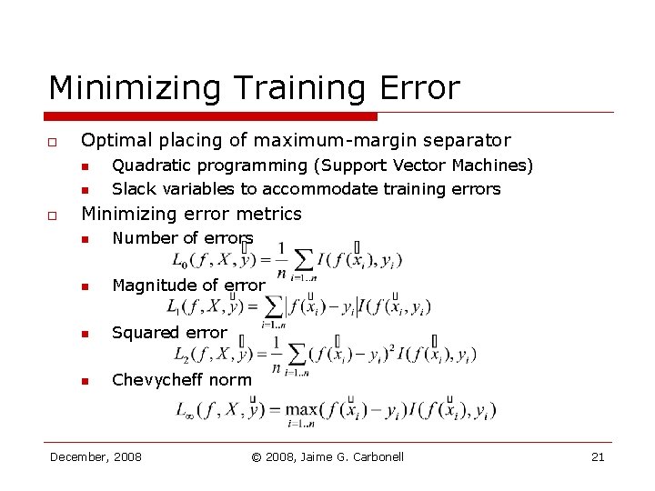
Minimizing Training Error o Optimal placing of maximum-margin separator n n o Quadratic programming (Support Vector Machines) Slack variables to accommodate training errors Minimizing error metrics n Number of errors n Magnitude of error n Squared error n Chevycheff norm December, 2008 © 2008, Jaime G. Carbonell 21
Symbolic Rule Induction General idea o Labeled instances are DB tuples o Rules are generalized tuples o Generalization occurs at terms in tuples o Generalize on new E+ not correctly predicted o Specialize on new E- not correctly predicted o Ignore predicted E+ or E- (error-driven learning) December, 2008 © 2008, Jaime G. Carbonell 22
Symbolic Rule Induction (2) Example term generalizations o Constant => disjunction e. g. if small portion value set seen o Constant => least-common-generalizer class e. g. if large portion of value set seen o Number (or ordinal) => range e. g. if dense sequential sampling December, 2008 © 2008, Jaime G. Carbonell 23
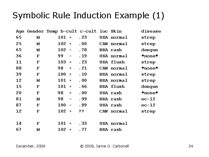
Symbolic Rule Induction Example (1) Age Gender Temp b-cult 65 M 101 + 25 M 102 + 65 M 102 36 F 99 11 F 103 + 88 F 98 + 39 F 100 + 12 M 101 + 15 F 101 + 20 F 98 + 81 M 98 87 F 100 12 F 102 + c-cult. 23. 00. 78. 19. 23. 21. 10. 00. 66. 00. 99. 89 ? ? loc USA CAN BRA BRA USA CAN 14 67 . 33. 77 USA normal BRA rash F M December, 2008 101 + 102 + Skin normal rash normal flush normal flush rash normal © 2008, Jaime G. Carbonell disease strep dengue *none* strep dengue *none* ec-12 strep 24
![Symbolic Rule Induction Example (2) Candidate Rules: IF age = [12, 65] gender = Symbolic Rule Induction Example (2) Candidate Rules: IF age = [12, 65] gender =](http://slidetodoc.com/presentation_image_h2/032abf1a98a880dfead4cec596820e5e/image-25.jpg)
Symbolic Rule Induction Example (2) Candidate Rules: IF age = [12, 65] gender = *any* temp = [100, 103] b-cult = + c-cult = [. 00, . 23] loc = *any* skin = (normal, flush) THEN: strep Disclaimer: These are not real medical records or rules IF age = (15, 65) gender = *any* temp = [101, 102] b-cult = *any* c-cult = [. 66, . 78] loc = BRA skin = rash THEN: dengue December, 2008 © 2008, Jaime G. Carbonell 25
Types of Data Mining o o “Supervised” Methods (this DM course) n Training data has both predictor attributes & objective (to be predicted) attributes n Predict discrete classes classification n Predict continuous values regression n Duality: classification regression “Unsupervised” Methods n Training data without objective attributes n Goal: find novel & interesting patterns n Cutting-edge research, fewer success stories n Semi-supervised methods: market-basket, … December, 2008 © 2008, Jaime G. Carbonell 26
Machine Learning Application Process in a Nutshell o o o Choose problem where n Prediction is valuable and non-trivial n Sufficient historical data is available n The objective is measurable (incl in past data) Prepare the data n Tabular form, clean, divide training & test sets Select a Machine Learning algorithm n Human readable decision fn rules, trees, … n Robust with noisy data k. NN, logistic reg, … December, 2008 © 2008, Jaime G. Carbonell 27
Machine Learning Application Process in a Nutshell (2) o o o Train ML Algorithm on Training Data Set n Each ML method has different training process n Training uses both predictor & objective att’s Run Training ML Algorithm on Test Data Set n Test uses only predictor att’s & outputs predictions on objective attributes n Compare predictions vs actual objective att’s (see lecture 2 for evaluation metrics) If Accuracy threshold, done. n Else, try different ML algorithm, different parameter settings, get more training data, … December, 2008 © 2008, Jaime G. Carbonell 28
![Sample DB Table (same) [predictor attributes] [objective] Tot Num Max Num Acct. Income Job Sample DB Table (same) [predictor attributes] [objective] Tot Num Max Num Acct. Income Job](http://slidetodoc.com/presentation_image_h2/032abf1a98a880dfead4cec596820e5e/image-29.jpg)
Sample DB Table (same) [predictor attributes] [objective] Tot Num Max Num Acct. Income Job Delinq Owns Credit Good numb. in K/yr Now? accts cycles home? years cust. ? -------------------------------------1001 85 Y 1 1 N 2 Y 1002 60 Y 3 2 Y 5 N 1003 ? N 0 0 N 2 N 1004 95 Y 1 2 N 9 Y 1005 100 Y 1 6 Y 3 Y 1006 29 Y 2 1 Y 1 N 1007 88 Y 6 4 Y 8 N 1008 80 Y 0 Y 1009 31 Y 1 1 N 1 Y 1011 ? Y ? 0 ? 7 Y 1012 75 ? 2 4 N 2 N 1013 20 N 1 1 N 3 N 1014 65 Y 1 3 Y 1015 65 N 1 2 N 8 Y 1016 20 N 0 N 1017 75 Y 1 3 N 2 N 1018 40 N 0 0 Y 10 Y December, 2008 © 2008, Jaime G. Carbonell 29
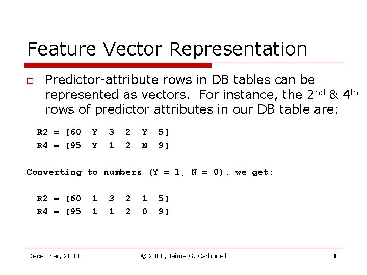
Feature Vector Representation o Predictor-attribute rows in DB tables can be represented as vectors. For instance, the 2 nd & 4 th rows of predictor attributes in our DB table are: R 2 = [60 R 4 = [95 Y Y 3 1 2 2 Y N 5] 9] Converting to numbers (Y = 1, N = 0), we get: R 2 = [60 R 4 = [95 December, 2008 1 1 3 1 2 2 1 0 5] 9] © 2008, Jaime G. Carbonell 30
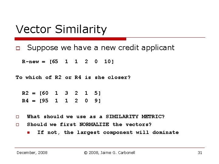
Vector Similarity o Suppose we have a new credit applicant R-new = [65 1 1 2 0 10] To which of R 2 or R 4 is she closer? R 2 = [60 R 4 = [95 o o 1 1 3 1 2 2 1 0 5] 9] What should we use as a SIMILARITY METRIC? Should we first NORMALIZE the vectors? n If not, the largest component will dominate December, 2008 © 2008, Jaime G. Carbonell 31
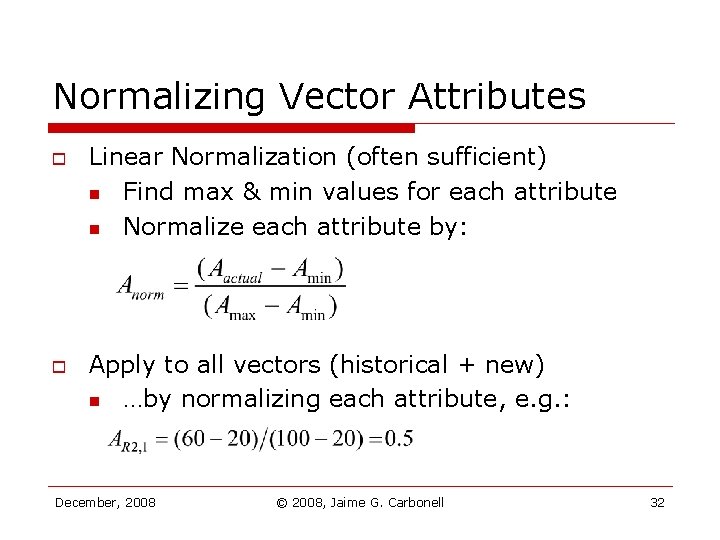
Normalizing Vector Attributes o o Linear Normalization (often sufficient) n Find max & min values for each attribute n Normalize each attribute by: Apply to all vectors (historical + new) n …by normalizing each attribute, e. g. : December, 2008 © 2008, Jaime G. Carbonell 32
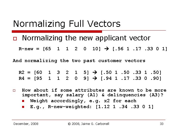
Normalizing Full Vectors o Normalizing the new applicant vector R-new = [65 1 1 2 0 10] [. 56 1. 17. 33 0 1] And normalizing the two past customer vectors R 2 = [60 R 4 = [95 o 1 1 3 1 2 2 1 0 5] [. 50 1. 50. 33 1. 50] 9] [. 94 1. 17. 33 0. 90] How about if some attributes are known to be more important, say salary (A 1) & delinquencies (A 3)? n Weight accordingly, e. g. x 2 for each n E. g. , R-new-weighted: [1. 12 1. 34. 33 0 1] December, 2008 © 2008, Jaime G. Carbonell 33
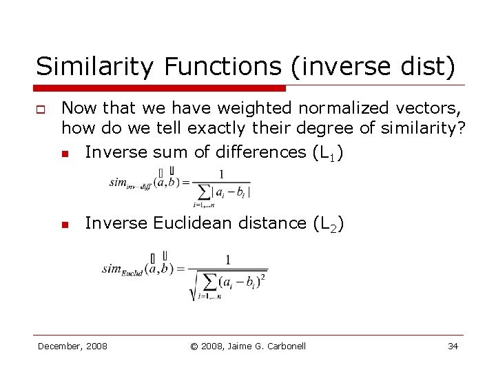
Similarity Functions (inverse dist) o Now that we have weighted normalized vectors, how do we tell exactly their degree of similarity? n Inverse sum of differences (L 1) n Inverse Euclidean distance (L 2) December, 2008 © 2008, Jaime G. Carbonell 34
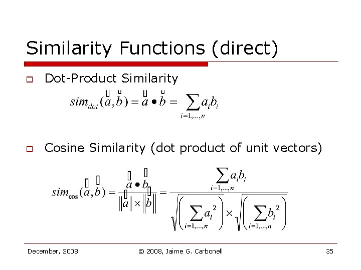
Similarity Functions (direct) o Dot-Product Similarity o Cosine Similarity (dot product of unit vectors) December, 2008 © 2008, Jaime G. Carbonell 35
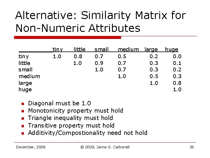
Alternative: Similarity Matrix for Non-Numeric Attributes tiny little small medium large huge n n n tiny 1. 0 little 0. 8 1. 0 small 0. 7 0. 9 1. 0 medium 0. 5 0. 7 1. 0 large 0. 2 0. 3 0. 5 1. 0 huge 0. 0 0. 1 0. 2 0. 3 0. 8 1. 0 Diagonal must be 1. 0 Monotonicity property must hold Triangle inequality must hold Transitive property must hold Additivity/Compostionality need not hold December, 2008 © 2008, Jaime G. Carbonell 36
k-Nearest Neighbors Method o o No explicit “training” phase When new case arrives (vector of predictor att’s) n Find nearest k neighbors (max similarity) among previous cases (row vectors in DB table) n k-neighbors vote for objective attribute o Unweighted majority vote, or o Similarity-weighted vote n Works for both discrete or continuous objective attributes December, 2008 © 2008, Jaime G. Carbonell 37
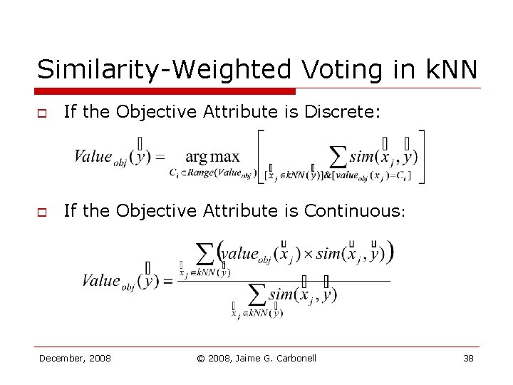
Similarity-Weighted Voting in k. NN o If the Objective Attribute is Discrete: o If the Objective Attribute is Continuous: December, 2008 © 2008, Jaime G. Carbonell 38
Applying k. NN to Real Problems 1 o o o How does one choose the vector representation? n Easy: Vector = predictor attributes What if attributes are not numerical? n Convert: (e. g. High=2, Med=1, Low=0), n Or, use similarity function over nominal values o E. g. equality or edit-distance on strings How does one choose a distance function? n Hard: No magic recipe; try simpler ones first n This implies a need for systematic testing (discussed in coming slides) December, 2008 © 2008, Jaime G. Carbonell 39
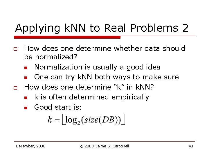
Applying k. NN to Real Problems 2 o o How does one determine whether data should be normalized? n Normalization is usually a good idea n One can try k. NN both ways to make sure How does one determine “k” in k. NN? n k is often determined empirically n Good start is: December, 2008 © 2008, Jaime G. Carbonell 40
Evaluating Machine Learning o o o Accuracy = Correct-Predictions/Total-Predictions n Simplest & most popular metric n But misleading on very-rare event prediction Precision, recall & F 1 n Borrowed from Information Retrieval n Applicable to very-rare event prediction Correlation (between predicted & actual values) for continuous objective attributes n R 2, kappa-coefficient, … December, 2008 © 2008, Jaime G. Carbonell 41
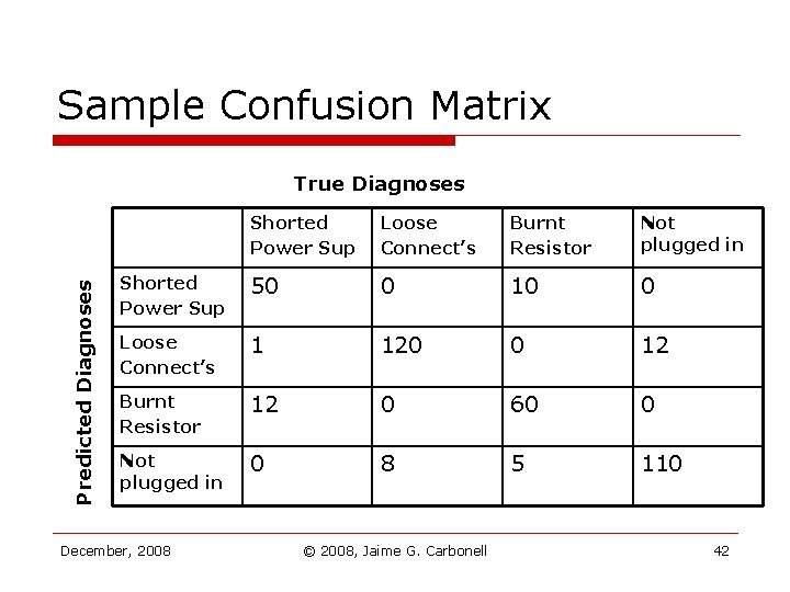
Sample Confusion Matrix Predicted Diagnoses True Diagnoses Shorted Power Sup Loose Connect’s Burnt Resistor Not plugged in Shorted Power Sup 50 0 10 0 Loose Connect’s 1 120 0 12 Burnt Resistor 12 0 60 0 Not plugged in 0 8 5 110 December, 2008 © 2008, Jaime G. Carbonell 42
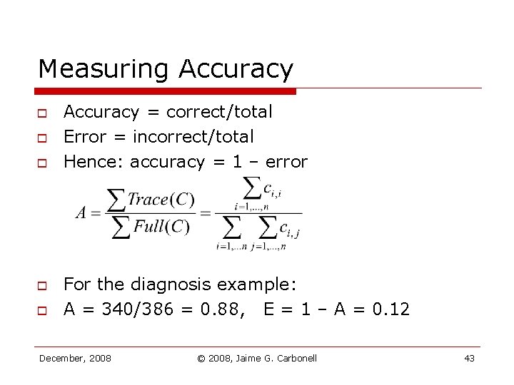
Measuring Accuracy o o o Accuracy = correct/total Error = incorrect/total Hence: accuracy = 1 – error For the diagnosis example: A = 340/386 = 0. 88, E = 1 – A = 0. 12 December, 2008 © 2008, Jaime G. Carbonell 43
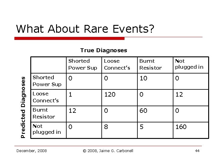
What About Rare Events? Predicted Diagnoses True Diagnoses Shorted Power Sup Loose Connect’s Burnt Resistor Not plugged in Shorted Power Sup 0 0 10 0 Loose Connect’s 1 120 0 12 Burnt Resistor 12 0 60 0 Not plugged in 0 8 5 160 December, 2008 © 2008, Jaime G. Carbonell 44
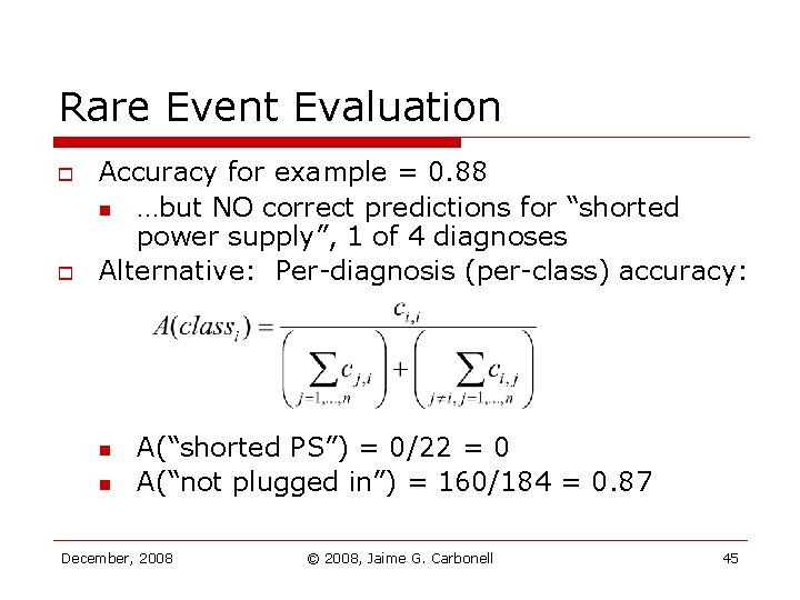
Rare Event Evaluation o o Accuracy for example = 0. 88 n …but NO correct predictions for “shorted power supply”, 1 of 4 diagnoses Alternative: Per-diagnosis (per-class) accuracy: n n A(“shorted PS”) = 0/22 = 0 A(“not plugged in”) = 160/184 = 0. 87 December, 2008 © 2008, Jaime G. Carbonell 45
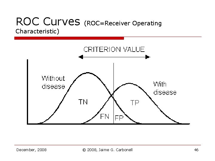
ROC Curves (ROC=Receiver Operating Characteristic) December, 2008 © 2008, Jaime G. Carbonell 46
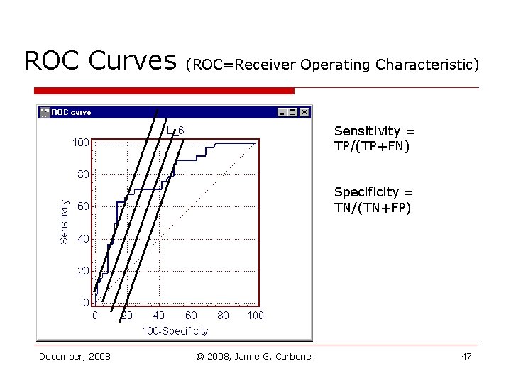
ROC Curves (ROC=Receiver Operating Characteristic) Sensitivity = TP/(TP+FN) Specificity = TN/(TN+FP) December, 2008 © 2008, Jaime G. Carbonell 47
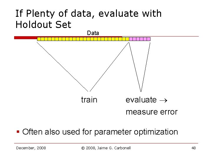
If Plenty of data, evaluate with Holdout Set Data train evaluate measure error § Often also used for parameter optimization December, 2008 © 2008, Jaime G. Carbonell 48
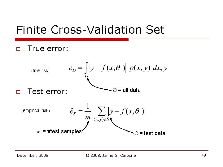
Finite Cross-Validation Set o True error: (true risk) o Test error: D = all data (empirical risk) m = #test samples December, 2008 S = test data © 2008, Jaime G. Carbonell 49
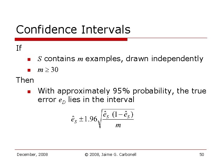
Confidence Intervals If n n S contains m examples, drawn independently m 30 Then n With approximately 95% probability, the true error e. D lies in the interval December, 2008 © 2008, Jaime G. Carbonell 50
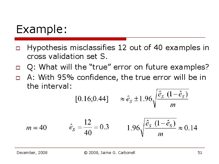
Example: o o o Hypothesis misclassifies 12 out of 40 examples in cross validation set S. Q: What will the “true” error on future examples? A: With 95% confidence, the true error will be in the interval: December, 2008 © 2008, Jaime G. Carbonell 51
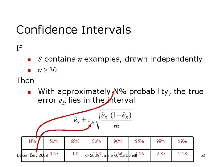
Confidence Intervals If n n S contains n examples, drawn independently n 30 Then n With approximately N% probability, the true error e. D lies in the interval N% 50% 68% z. N 2008 December, 0. 67 1. 0 80% 95% 98% 99% 1. 28 Jaime 1. 64 © 2008, G. Carbonell 1. 96 2. 33 2. 58 52
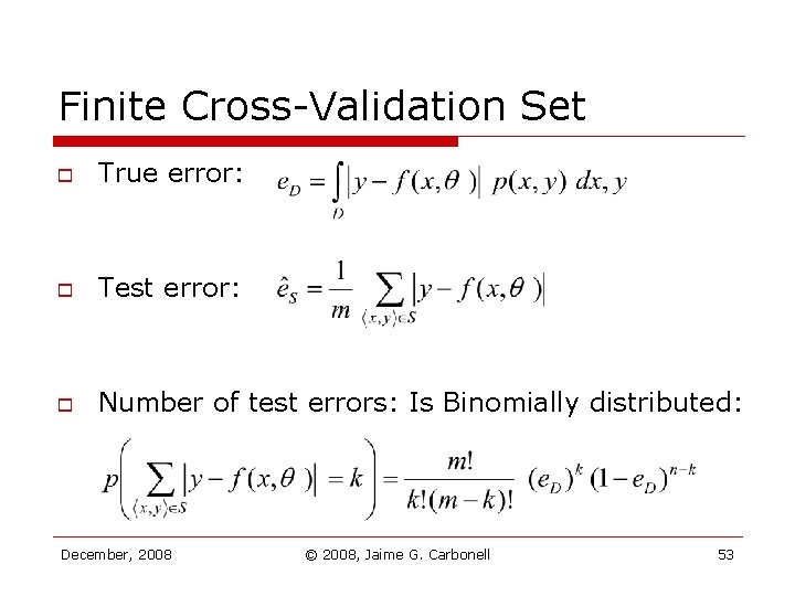
Finite Cross-Validation Set o True error: o Test error: o Number of test errors: Is Binomially distributed: December, 2008 © 2008, Jaime G. Carbonell 53
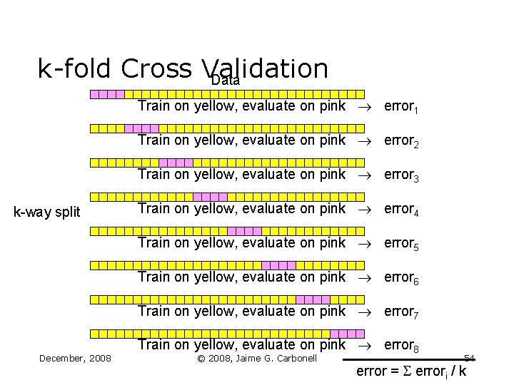
k-fold Cross Validation Data Train on yellow, evaluate on pink error 1 Train on yellow, evaluate on pink error 2 Train on yellow, evaluate on pink error 3 k-way split Train on yellow, evaluate on pink error 4 Train on yellow, evaluate on pink error 5 Train on yellow, evaluate on pink error 6 Train on yellow, evaluate on pink error 7 December, 2008 Train on yellow, evaluate on pink error 8 © 2008, Jaime G. Carbonell 54 error = errori / k
Cross Validation Procedure o o o Purpose: Evaluate DM accuracy on training data Experiment: Try different similarity functions, etc. Process: n Divide the training data into k equal pieces (each piece is called a “fold”) n Train the classifier using all but kth fold n Test for accuracy on kth fold n Repeat with kth-1 fold held out for testing, then with kth-2 fold for testing, till tested on all folds n Report the average accuracy across folds December, 2008 © 2008, Jaime G. Carbonell 55
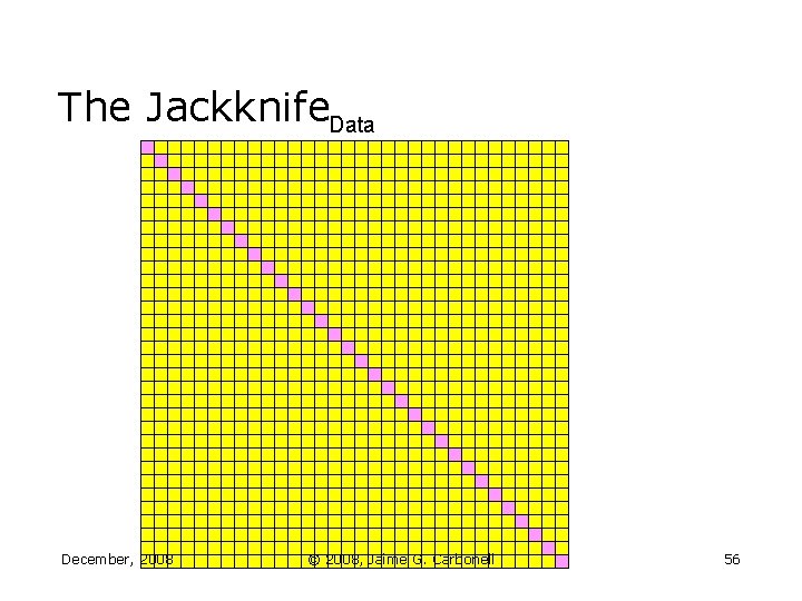
The Jackknife. Data December, 2008 © 2008, Jaime G. Carbonell 56
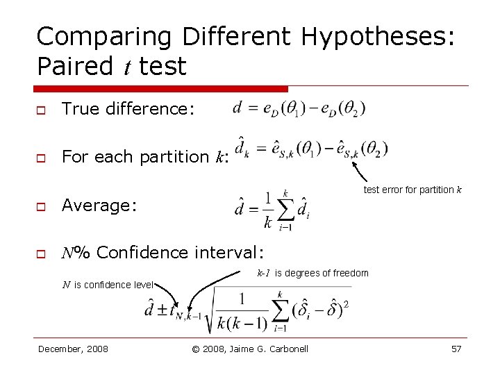
Comparing Different Hypotheses: Paired t test o True difference: o For each partition k: test error for partition k o Average: o N% Confidence interval: k-1 is degrees of freedom N is confidence level December, 2008 © 2008, Jaime G. Carbonell 57
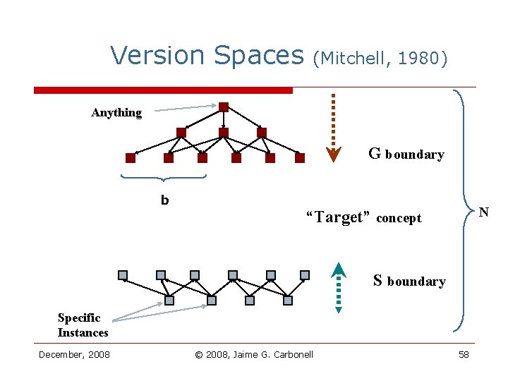
Version Spaces (Mitchell, 1980) Anything G boundary b N “Target” concept S boundary Specific Instances December, 2008 © 2008, Jaime G. Carbonell 58
Original & Seeded Version Spaces o o Version-spaces (Mitchell, 1980) n Symbolic multivariate learning n S & G sets define lattice boundaries n Exponential worst-case: O(b. N) Seeded Version Spaces (Carbonell, 2002) n Generality level hypothesis seed n S & G subsets effective lattice n Polynomial worst case: O(bk/2), k=3, 4 December, 2008 © 2008, Jaime G. Carbonell 59
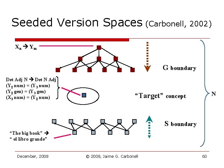
Seeded Version Spaces (Carbonell, 2002) Xn Ym G boundary Det Adj N Det N Adj (Y 2 num) = (Y 3 num) (Y 2 gen) = (Y 3 gen) (X 3 num) = (Y 2 num) N “Target” concept S boundary “The big book” “ el libro grande” December, 2008 © 2008, Jaime G. Carbonell 60
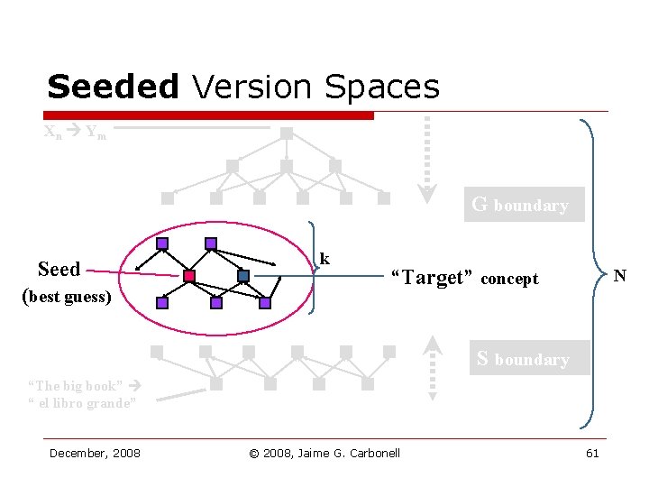
Seeded Version Spaces Xn Ym G boundary Seed (best guess) k “Target” concept N S boundary “The big book” “ el libro grande” December, 2008 © 2008, Jaime G. Carbonell 61
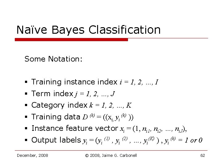
Naïve Bayes Classification Some Notation: § Training instance index i = 1, 2, …, I § Term index j = 1, 2, …, J § Category index k = 1, 2, …, K § Training data D (k) = ((xi, yi (k) )) § Instance feature vector xi = (1, ni 2, …, ni. J), § Output labels yi = (yi (1) , yi (2) , …, yi(K) ) , yi (k) = 1 or 0 December, 2008 © 2008, Jaime G. Carbonell 62
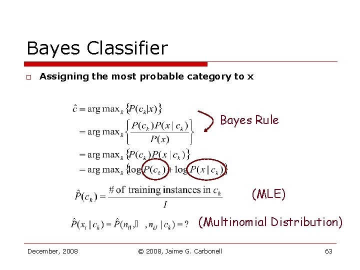
Bayes Classifier o Assigning the most probable category to x Bayes Rule (MLE) (Multinomial Distribution) December, 2008 © 2008, Jaime G. Carbonell 63
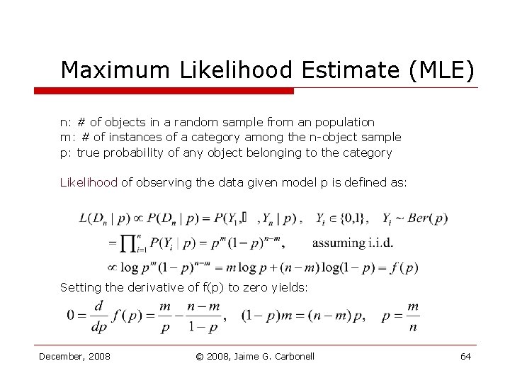
Maximum Likelihood Estimate (MLE) n: # of objects in a random sample from an population m: # of instances of a category among the n-object sample p: true probability of any object belonging to the category Likelihood of observing the data given model p is defined as: Setting the derivative of f(p) to zero yields: December, 2008 © 2008, Jaime G. Carbonell 64
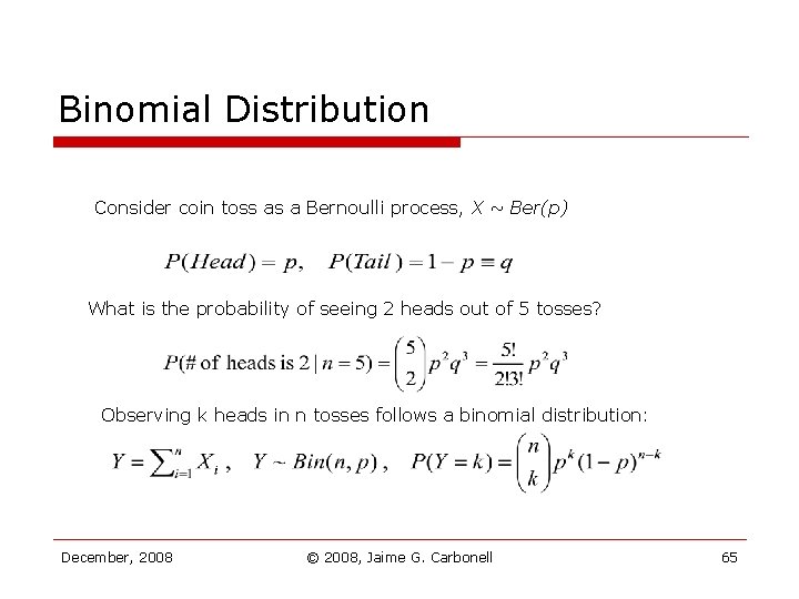
Binomial Distribution Consider coin toss as a Bernoulli process, X ~ Ber(p) What is the probability of seeing 2 heads out of 5 tosses? Observing k heads in n tosses follows a binomial distribution: December, 2008 © 2008, Jaime G. Carbonell 65
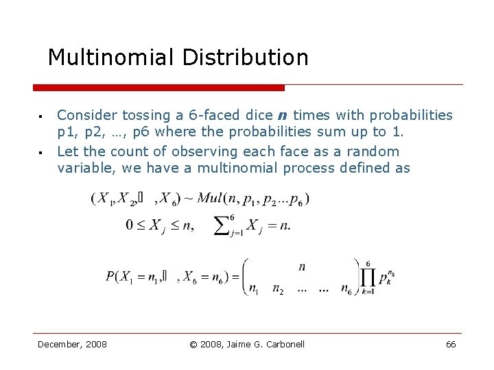
Multinomial Distribution § § Consider tossing a 6 -faced dice n times with probabilities p 1, p 2, …, p 6 where the probabilities sum up to 1. Let the count of observing each face as a random variable, we have a multinomial process defined as December, 2008 © 2008, Jaime G. Carbonell 66
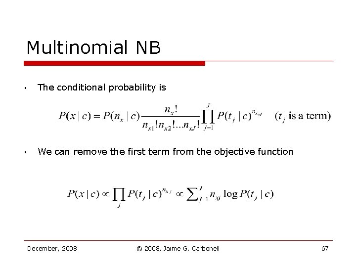
Multinomial NB § The conditional probability is § We can remove the first term from the objective function December, 2008 © 2008, Jaime G. Carbonell 67
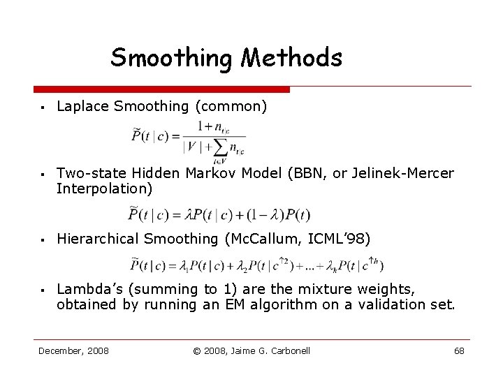
Smoothing Methods § § Laplace Smoothing (common) Two-state Hidden Markov Model (BBN, or Jelinek-Mercer Interpolation) Hierarchical Smoothing (Mc. Callum, ICML’ 98) Lambda’s (summing to 1) are the mixture weights, obtained by running an EM algorithm on a validation set. December, 2008 © 2008, Jaime G. Carbonell 68
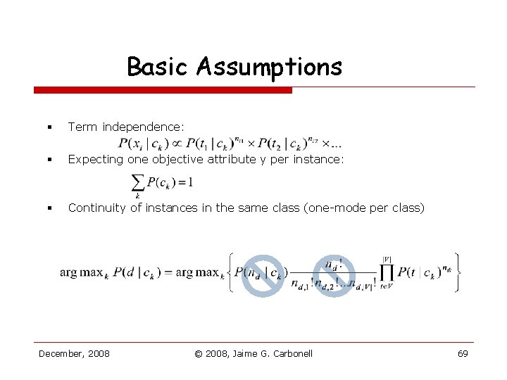
Basic Assumptions § Term independence: § Expecting one objective attribute y per instance: § Continuity of instances in the same class (one-mode per class) December, 2008 © 2008, Jaime G. Carbonell 69
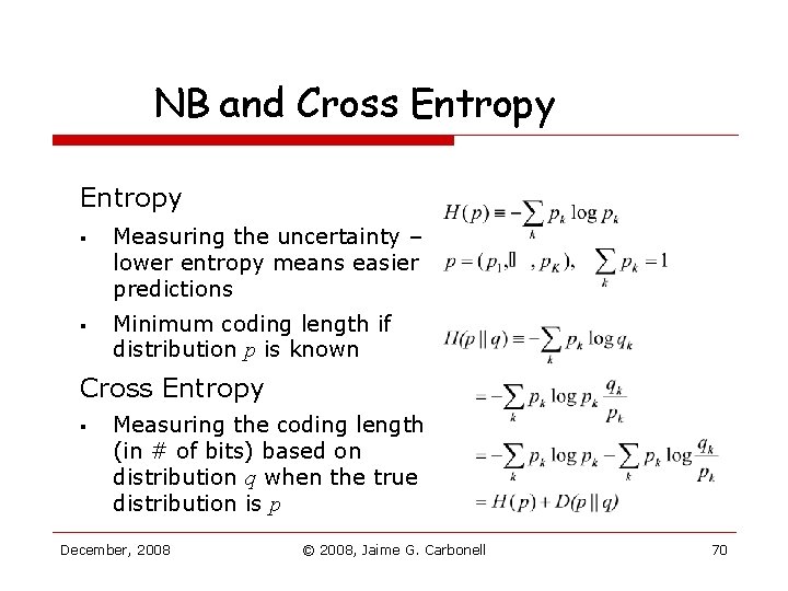
NB and Cross Entropy § § Measuring the uncertainty – lower entropy means easier predictions Minimum coding length if distribution p is known Cross Entropy § Measuring the coding length (in # of bits) based on distribution q when the true distribution is p December, 2008 © 2008, Jaime G. Carbonell 70
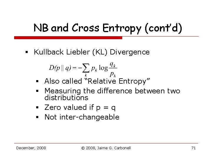
NB and Cross Entropy (cont’d) § Kullback Liebler (KL) Divergence § Also called “Relative Entropy” § Measuring the difference between two distributions § Zero valued if p = q § Not inter-changeable December, 2008 © 2008, Jaime G. Carbonell 71
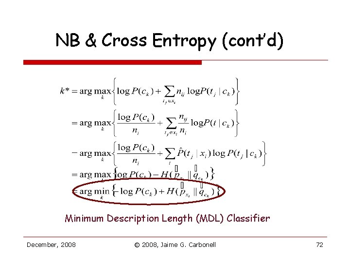
NB & Cross Entropy (cont’d) Minimum Description Length (MDL) Classifier December, 2008 © 2008, Jaime G. Carbonell 72
Concluding Remarks on NB Pros § Explicit probabilistic reasoning § Relatively effective, fast online response (as an eager learning) Cons § § § Scoring function (logarithm of term probabilities) would be too sensitive to measurement errors on rare features One-class-per-instance assumption imposes both theoretical and practical limitations Empirically weak when dealing with rare categories and large feature sets December, 2008 © 2008, Jaime G. Carbonell 73
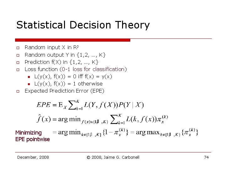
Statistical Decision Theory o o o Random input X in RJ Random output Y in {1, 2, …, K} Prediction f(X) in {1, 2, …, K} Loss function (0 -1 loss for classification) n L(y(x), f(x)) = 0 iff f(x) = y(x) n L(y(x), f(x)) = 1 otherwise Expected Prediction Error (EPE) Minimizing EPE pointwise December, 2008 © 2008, Jaime G. Carbonell 74
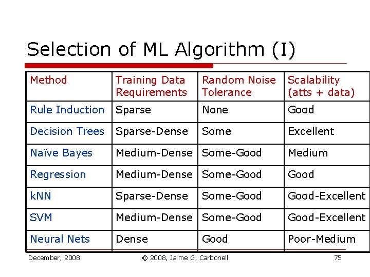
Selection of ML Algorithm (I) Method Training Data Requirements Random Noise Tolerance Scalability (atts + data) Rule Induction Sparse None Good Decision Trees Sparse-Dense Some Excellent Naïve Bayes Medium-Dense Some-Good Medium Regression Medium-Dense Some-Good k. NN Sparse-Dense Some-Good-Excellent SVM Medium-Dense Some-Good-Excellent Neural Nets Dense Poor-Medium December, 2008 Good © 2008, Jaime G. Carbonell 75
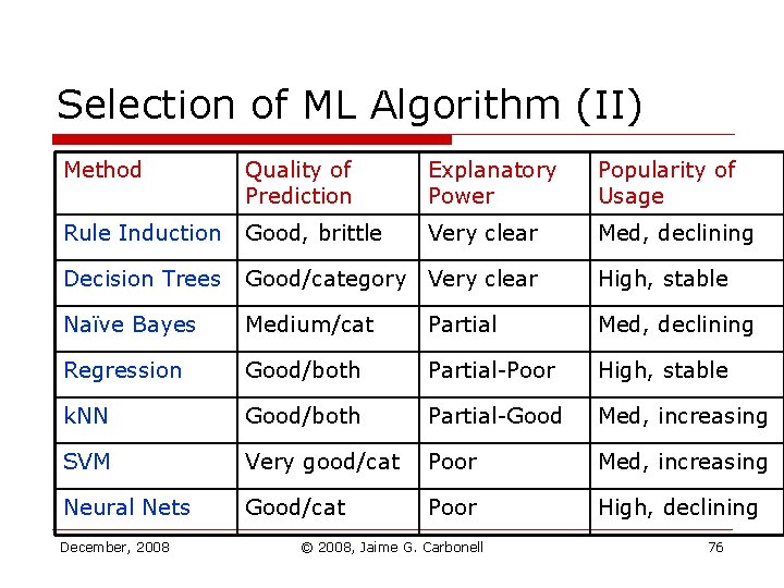
Selection of ML Algorithm (II) Method Quality of Prediction Explanatory Power Popularity of Usage Rule Induction Good, brittle Very clear Med, declining Decision Trees Good/category Very clear High, stable Naïve Bayes Medium/cat Partial Med, declining Regression Good/both Partial-Poor High, stable k. NN Good/both Partial-Good Med, increasing SVM Very good/cat Poor Med, increasing Neural Nets Good/cat Poor High, declining December, 2008 © 2008, Jaime G. Carbonell 76
- Slides: 76