Machine Learning Data Mining CSCNSEE 155 Lecture 10

Machine Learning & Data Mining CS/CNS/EE 155 Lecture 10: Boosting & Ensemble Selection 1

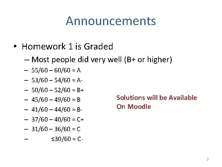
Announcements • Homework 1 is Graded – Most people did very well (B+ or higher) – – – – 55/60 – 60/60 ≈ A 53/60 – 54/60 ≈ A 50/60 – 52/60 ≈ B+ 45/60 – 49/60 ≈ B 41/60 – 44/60 ≈ B 37/60 – 40/60 ≈ C+ 31/60 – 36/60 ≈ C ≤ 30/60 ≈ C- Solutions will be Available On Moodle 2

Kaggle Mini-Project • Small bug in data file – Was fixed this morning. – So if you downloaded already, download again. • Finding Group Members – Offices hours today, mingle in person – Online signup sheet later 3

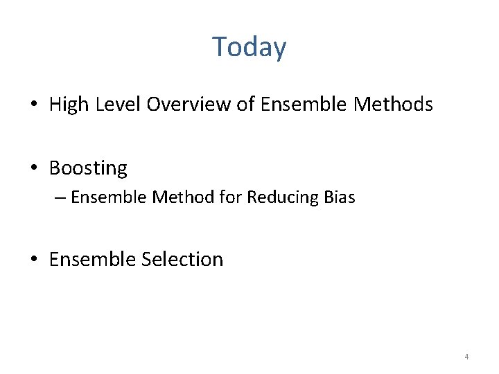
Today • High Level Overview of Ensemble Methods • Boosting – Ensemble Method for Reducing Bias • Ensemble Selection 4

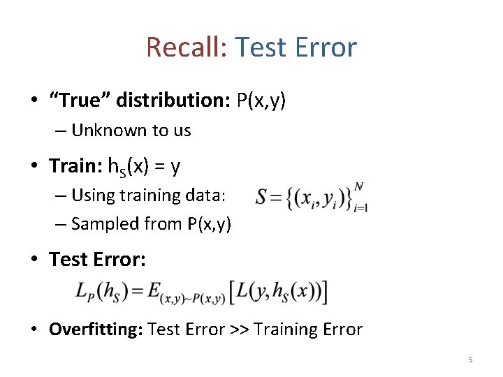
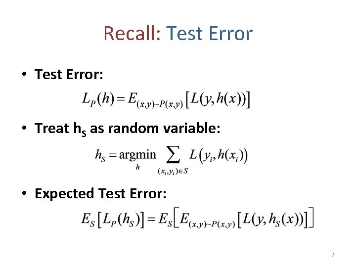
Recall: Test Error • “True” distribution: P(x, y) – Unknown to us • Train: h. S(x) = y – Using training data: – Sampled from P(x, y) • Test Error: • Overfitting: Test Error >> Training Error 5

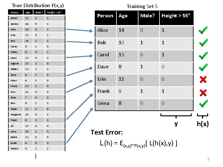
True Distribution P(x, y) Person Age Male? Height > 55” James 11 1 1 Jessica 14 0 1 Alice 14 0 1 Amy 12 0 1 Bob 10 1 1 Xavier 9 1 0 Cathy 9 0 1 Carol 13 0 1 Eugene 13 1 0 Rafael 12 1 1 Dave 8 1 0 Peter 9 1 0 Henry 13 1 0 Erin 11 0 0 Rose 7 0 0 Iain 8 1 1 Paulo 12 1 0 Margaret 10 0 1 Frank 9 1 1 Jill 13 0 0 Leon 10 1 0 Sarah 12 0 0 Gena 8 0 0 Patrick 5 1 1 Training Set S Person Age Male? Height > 55” Alice 14 0 1 Bob 10 1 1 Carol 13 0 1 Dave 8 1 0 Erin 11 0 0 Frank 9 1 1 Gena 8 0 0 y Test Error: L(h) = E(x, y)~P(x, y)[ L(h(x), y) ] h(x) … 6

Recall: Test Error • Test Error: • Treat h. S as random variable: • Expected Test Error: 7

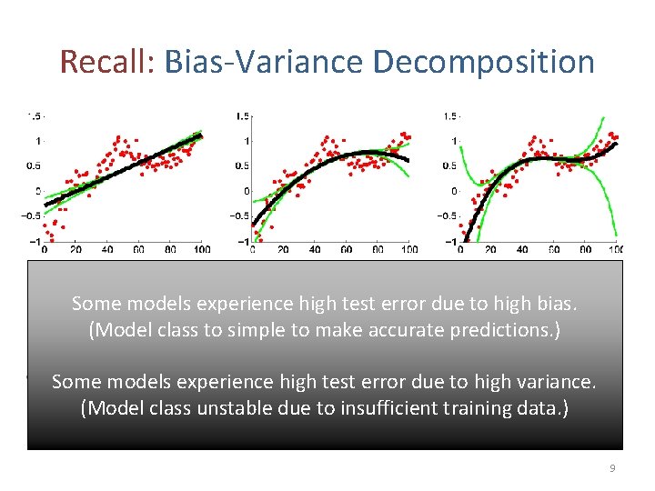
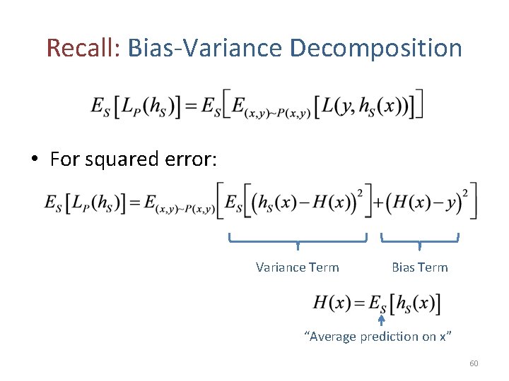
Recall: Bias-Variance Decomposition • For squared error: Variance Term Bias Term “Average prediction on x” 8

Recall: Bias-Variance Decomposition Bias models Variance Bias bias. Variance Bias test Some experience high error due to high (Model class to simple to make accurate predictions. ) Some models experience high test error due to high variance. (Model class unstable due to insufficient training data. ) 9

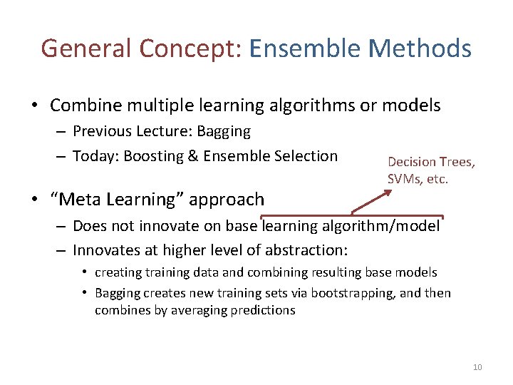
General Concept: Ensemble Methods • Combine multiple learning algorithms or models – Previous Lecture: Bagging – Today: Boosting & Ensemble Selection • “Meta Learning” approach Decision Trees, SVMs, etc. – Does not innovate on base learning algorithm/model – Innovates at higher level of abstraction: • creating training data and combining resulting base models • Bagging creates new training sets via bootstrapping, and then combines by averaging predictions 10

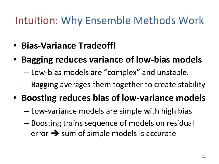
Intuition: Why Ensemble Methods Work • Bias-Variance Tradeoff! • Bagging reduces variance of low-bias models – Low-bias models are “complex” and unstable. – Bagging averages them together to create stability • Boosting reduces bias of low-variance models – Low-variance models are simple with high bias – Boosting trains sequence of models on residual error sum of simple models is accurate 11

Boosting “The Strength of Weak Classifiers”* * http: //www. cs. princeton. edu/~schapire/papers/strengthofweak. pdf 12

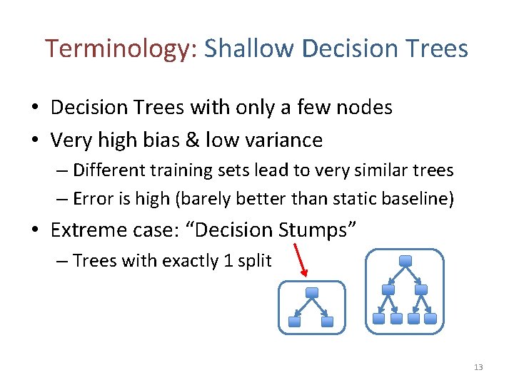
Terminology: Shallow Decision Trees • Decision Trees with only a few nodes • Very high bias & low variance – Different training sets lead to very similar trees – Error is high (barely better than static baseline) • Extreme case: “Decision Stumps” – Trees with exactly 1 split 13

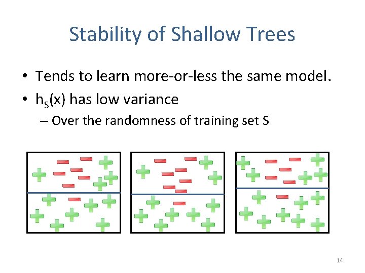
Stability of Shallow Trees • Tends to learn more-or-less the same model. • h. S(x) has low variance – Over the randomness of training set S 14

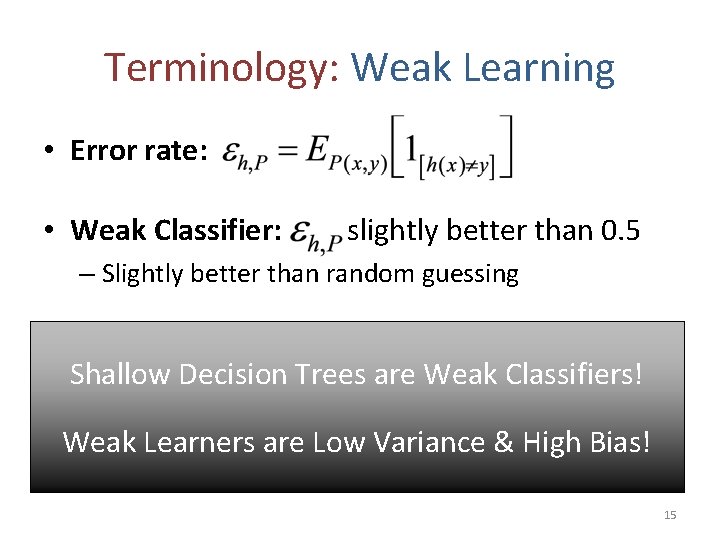
Terminology: Weak Learning • Error rate: • Weak Classifier: slightly better than 0. 5 – Slightly better than random guessing • Weak Learner: can learn a weak classifier Shallow Decision Trees are Weak Classifiers! Weak Learners are Low Variance & High Bias! 15

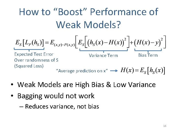
How to “Boost” Performance of Weak Models? Expected Test Error Variance Term Over randomness of S (Squared Loss) “Average prediction on x” Bias Term • Weak Models are High Bias & Low Variance • Bagging would not work – Reduces variance, not bias 16

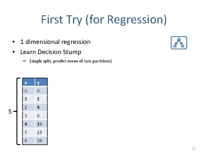
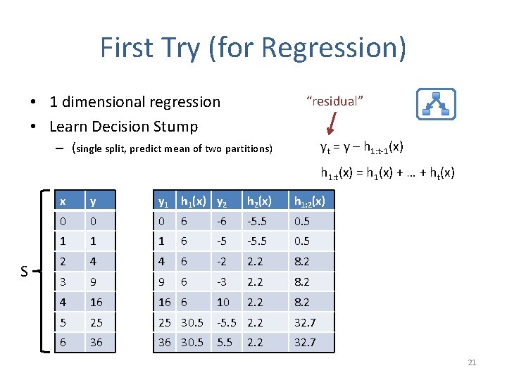
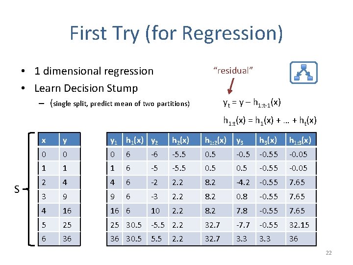
First Try (for Regression) • 1 dimensional regression • Learn Decision Stump – (single split, predict mean of two partitions) S x y 0 0 1 1 2 4 3 9 4 16 5 25 6 36 17

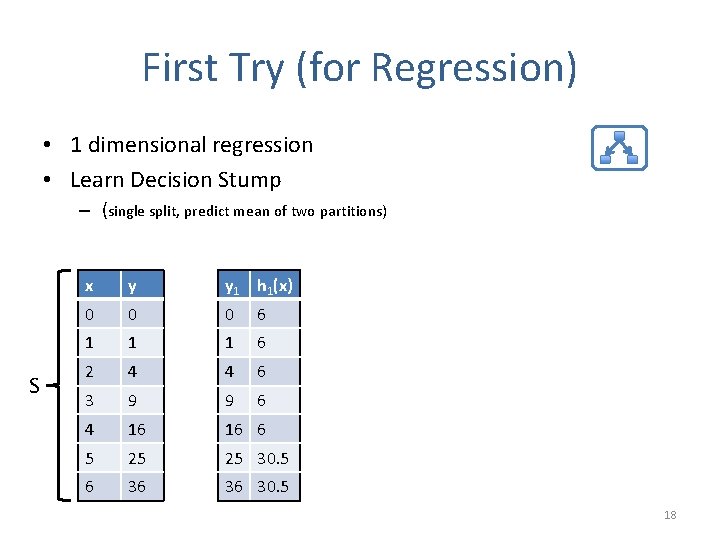
First Try (for Regression) • 1 dimensional regression • Learn Decision Stump – (single split, predict mean of two partitions) S x y y 1 h 1(x) 0 0 0 6 1 1 1 6 2 4 4 6 3 9 9 6 4 16 16 6 5 25 25 30. 5 6 36 36 30. 5 18

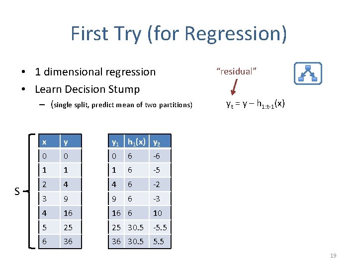
First Try (for Regression) • 1 dimensional regression • Learn Decision Stump – (single split, predict mean of two partitions) S x y y 1 h 1(x) y 2 0 0 0 6 -6 1 1 1 6 -5 2 4 4 6 -2 3 9 9 6 -3 4 16 16 6 10 5 25 25 30. 5 -5. 5 6 36 36 30. 5 5. 5 “residual” yt = y – h 1: t-1(x) 19

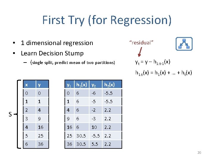
First Try (for Regression) • 1 dimensional regression • Learn Decision Stump “residual” – (single split, predict mean of two partitions) yt = y – h 1: t-1(x) h 1: t(x) = h 1(x) + … + ht(x) S x y y 1 h 1(x) y 2 h 2(x) 0 0 0 6 -6 -5. 5 1 1 1 6 -5 -5. 5 2 4 4 6 -2 2. 2 3 9 9 6 -3 2. 2 4 16 16 6 10 2. 2 5 25 25 30. 5 -5. 5 2. 2 6 36 36 30. 5 5. 5 2. 2 20

First Try (for Regression) • 1 dimensional regression • Learn Decision Stump “residual” yt = y – h 1: t-1(x) – (single split, predict mean of two partitions) h 1: t(x) = h 1(x) + … + ht(x) S x y y 1 h 1(x) y 2 h 2(x) h 1: 2(x) 0 0 0 6 -6 -5. 5 0. 5 1 1 1 6 -5 -5. 5 0. 5 2 4 4 6 -2 2. 2 8. 2 3 9 9 6 -3 2. 2 8. 2 4 16 16 6 10 2. 2 8. 2 5 25 25 30. 5 -5. 5 2. 2 32. 7 6 36 36 30. 5 5. 5 32. 7 2. 2 21

First Try (for Regression) • 1 dimensional regression • Learn Decision Stump “residual” yt = y – h 1: t-1(x) – (single split, predict mean of two partitions) h 1: t(x) = h 1(x) + … + ht(x) S x y y 1 h 1(x) y 2 h 2(x) h 1: 2(x) y 3 h 3(x) h 1: 3(x) 0 0 0 6 -6 -5. 5 0. 5 -0. 55 -0. 05 1 1 1 6 -5 -5. 5 0. 5 -0. 55 -0. 05 2 4 4 6 -2 2. 2 8. 2 -4. 2 -0. 55 7. 65 3 9 9 6 -3 2. 2 8. 2 0. 8 -0. 55 7. 65 4 16 16 6 10 2. 2 8. 2 7. 8 -0. 55 7. 65 5 25 25 30. 5 -5. 5 2. 2 32. 7 -7. 7 -0. 55 32. 15 6 36 36 30. 5 5. 5 32. 7 3. 3 36 2. 2 22

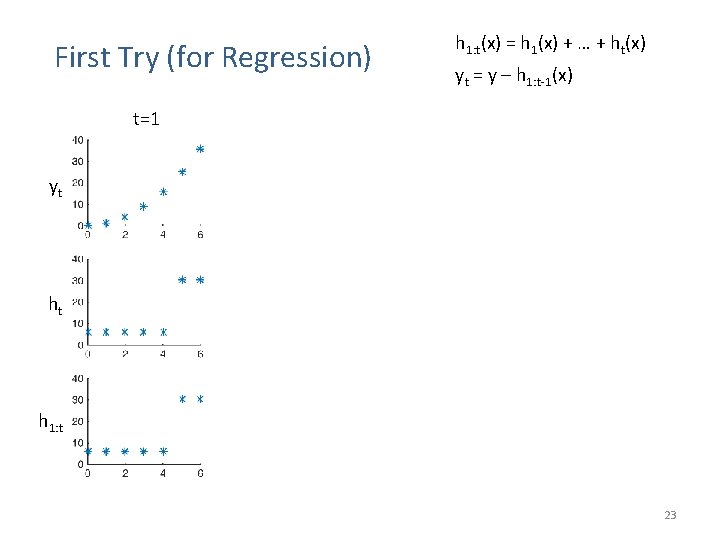
First Try (for Regression) t=1 t=2 h 1: t(x) = h 1(x) + … + ht(x) yt = y – h 1: t-1(x) t=3 t=4 yt ht h 1: t 23

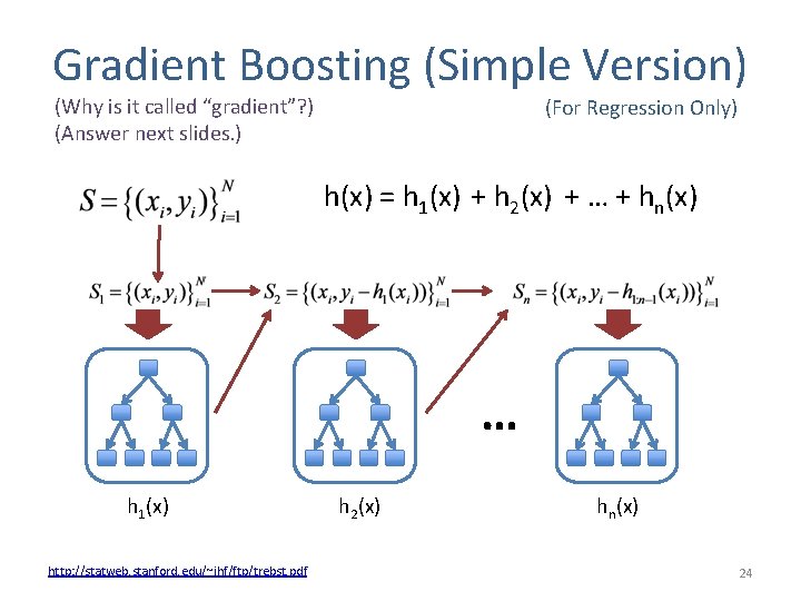
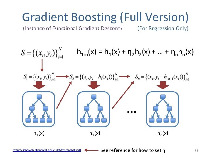
Gradient Boosting (Simple Version) (Why is it called “gradient”? ) (Answer next slides. ) (For Regression Only) h(x) = h 1(x) + h 2(x) + … + hn(x) … h 1(x) http: //statweb. stanford. edu/~jhf/ftp/trebst. pdf h 2(x) hn(x) 24

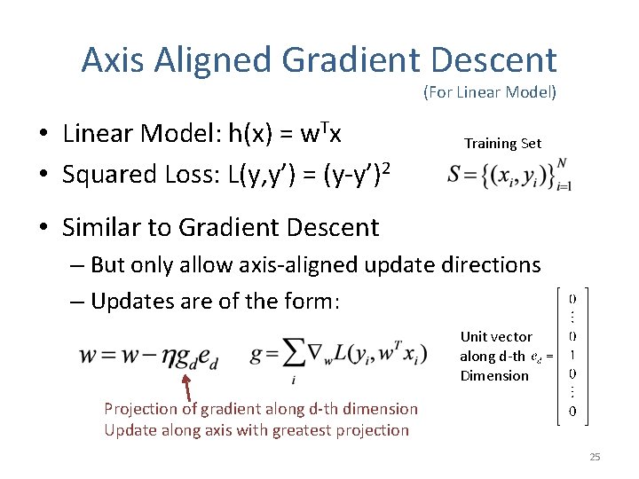
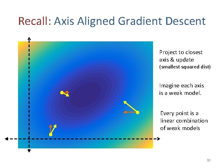
Axis Aligned Gradient Descent (For Linear Model) • Linear Model: h(x) = w. Tx • Squared Loss: L(y, y’) = (y-y’)2 Training Set • Similar to Gradient Descent – But only allow axis-aligned update directions – Updates are of the form: Unit vector along d-th Dimension Projection of gradient along d-th dimension Update along axis with greatest projection 25

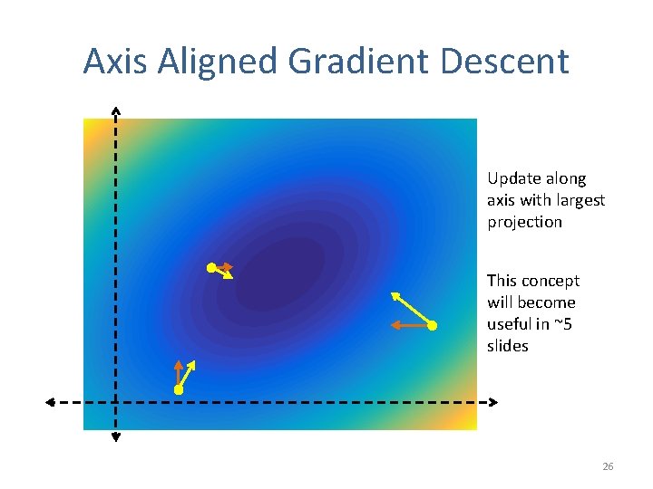
Axis Aligned Gradient Descent Update along axis with largest projection This concept will become useful in ~5 slides 26

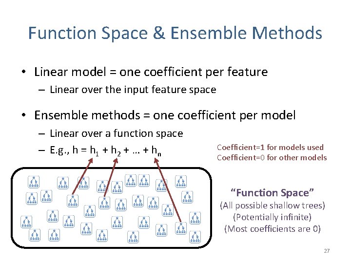
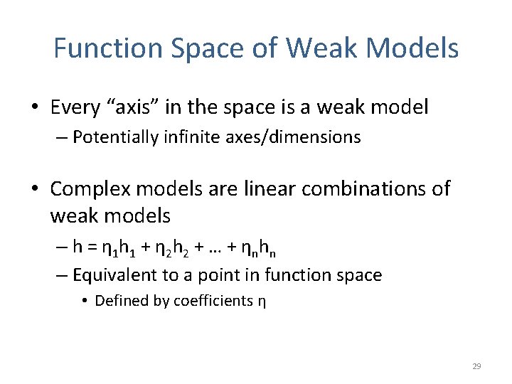
Function Space & Ensemble Methods • Linear model = one coefficient per feature – Linear over the input feature space • Ensemble methods = one coefficient per model – Linear over a function space – E. g. , h = h 1 + h 2 + … + hn Coefficient=1 for models used Coefficient=0 for other models “Function Space” (All possible shallow trees) (Potentially infinite) (Most coefficients are 0) 27

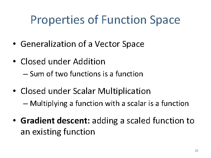
Properties of Function Space • Generalization of a Vector Space • Closed under Addition – Sum of two functions is a function • Closed under Scalar Multiplication – Multiplying a function with a scalar is a function • Gradient descent: adding a scaled function to an existing function 28

Function Space of Weak Models • Every “axis” in the space is a weak model – Potentially infinite axes/dimensions • Complex models are linear combinations of weak models – h = η 1 h 1 + η 2 h 2 + … + ηn h n – Equivalent to a point in function space • Defined by coefficients η 29

Recall: Axis Aligned Gradient Descent Project to closest axis & update (smallest squared dist) Imagine each axis is a weak model. Every point is a linear combination of weak models 30

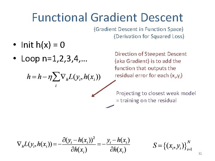
Functional Gradient Descent • Init h(x) = 0 • Loop n=1, 2, 3, 4, … (Gradient Descent in Function Space) (Derivation for Squared Loss) Direction of Steepest Descent (aka Gradient) is to add the function that outputs the residual error for each (xi, yi) Projecting to closest weak model = training on the residual 31

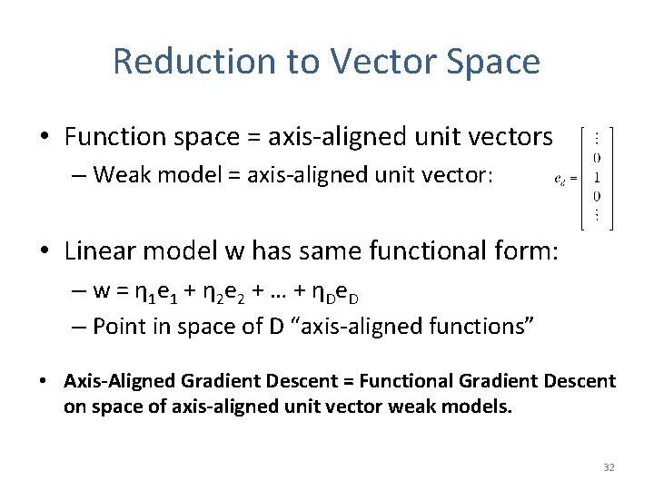
Reduction to Vector Space • Function space = axis-aligned unit vectors – Weak model = axis-aligned unit vector: • Linear model w has same functional form: – w = η 1 e 1 + η 2 e 2 + … + ηD e D – Point in space of D “axis-aligned functions” • Axis-Aligned Gradient Descent = Functional Gradient Descent on space of axis-aligned unit vector weak models. 32

Gradient Boosting (Full Version) (Instance of Functional Gradient Descent) (For Regression Only) h 1: n(x) = h 1(x) + η 2 h 2(x) + … + ηnhn(x) … h 1(x) http: //statweb. stanford. edu/~jhf/ftp/trebst. pdf h 2(x) hn(x) See reference for how to set η 33

Recap: Basic Boosting • Ensemble of many weak classifiers. – h(x) = η 1 h 1(x) +η 2 h 2(x) + … + ηnhn(x) • Goal: reduce bias using low-variance models • Derivation: via Gradient Descent in Function Space – Space of weak classifiers • We’ve only seen the regression so far… 34

Ada. Boost Adaptive Boosting for Classification http: //www. yisongyue. com/courses/cs 155/lectures/msri. pdf 35

Boosting for Classification • Gradient Boosting was designed for regression • Can we design one for classification? • Ada. Boost – Adaptive Boosting 36

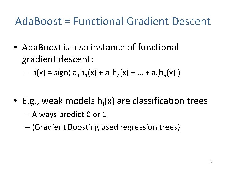
Ada. Boost = Functional Gradient Descent • Ada. Boost is also instance of functional gradient descent: – h(x) = sign( a 1 h 1(x) + a 2 h 2(x) + … + a 3 hn(x) ) • E. g. , weak models hi(x) are classification trees – Always predict 0 or 1 – (Gradient Boosting used regression trees) 37

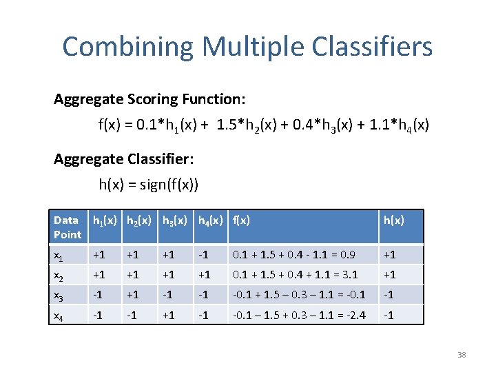
Combining Multiple Classifiers Aggregate Scoring Function: f(x) = 0. 1*h 1(x) + 1. 5*h 2(x) + 0. 4*h 3(x) + 1. 1*h 4(x) Aggregate Classifier: h(x) = sign(f(x)) Data h 1(x) h 2(x) h 3(x) h 4(x) f(x) Point h(x) x 1 +1 +1 +1 -1 0. 1 + 1. 5 + 0. 4 - 1. 1 = 0. 9 +1 x 2 +1 +1 0. 1 + 1. 5 + 0. 4 + 1. 1 = 3. 1 +1 x 3 -1 +1 -1 -1 -0. 1 + 1. 5 – 0. 3 – 1. 1 = -0. 1 -1 x 4 -1 -1 +1 -1 -0. 1 – 1. 5 + 0. 3 – 1. 1 = -2. 4 -1 38

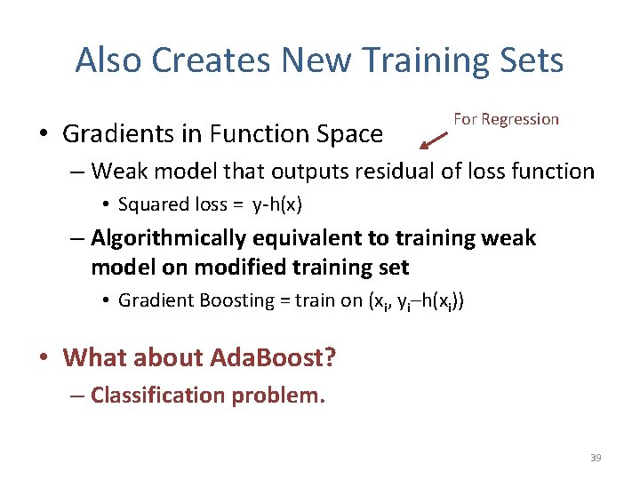
Also Creates New Training Sets • Gradients in Function Space For Regression – Weak model that outputs residual of loss function • Squared loss = y-h(x) – Algorithmically equivalent to training weak model on modified training set • Gradient Boosting = train on (xi, yi–h(xi)) • What about Ada. Boost? – Classification problem. 39

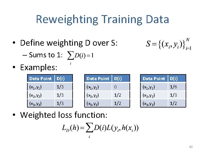
Reweighting Training Data • Define weighting D over S: – Sums to 1: • Examples: Data Point D(i) (x 1, y 1) 1/3 (x 1, y 1) 0 (x 1, y 1) 1/6 (x 2, y 2) 1/3 (x 2, y 2) 1/2 (x 2, y 2) 1/3 (x 3, y 3) 1/2 • Weighted loss function: 40

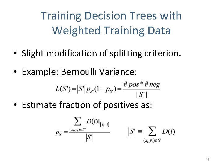
Training Decision Trees with Weighted Training Data • Slight modification of splitting criterion. • Example: Bernoulli Variance: • Estimate fraction of positives as: 41

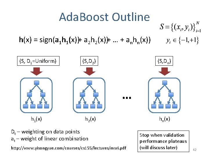
Ada. Boost Outline (x))+ … + anhn(x)) h(x) = sign(a 1 h 1(x) (x))+ a 2 h 2(x) (S, D 1=Uniform) (S, D 2) (S, Dn) … h 1(x) h 2(x) Dt – weighting on data points at – weight of linear combination http: //www. yisongyue. com/courses/cs 155/lectures/msri. pdf hn(x) Stop when validation performance plateaus (will discuss later) 42

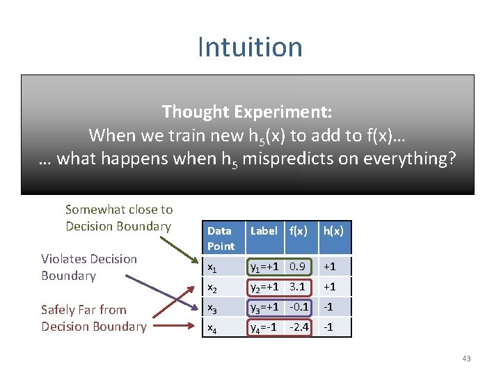
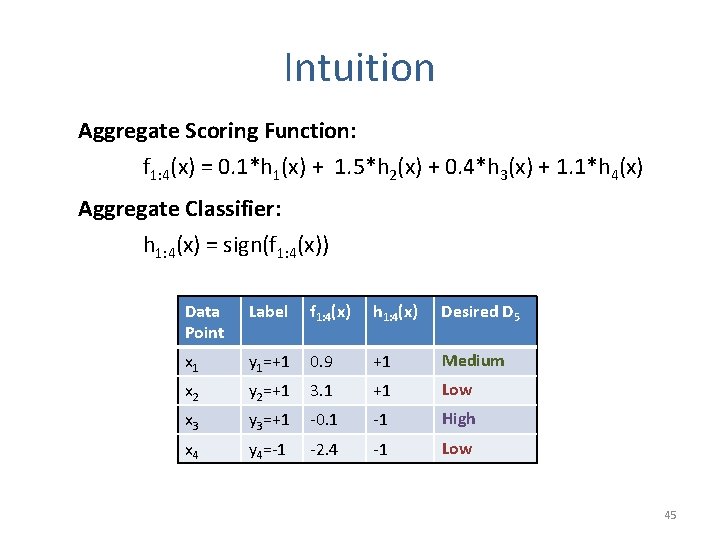
Intuition Aggregate Scoring Function: Thought Experiment: f(x) = 0. 1*h 1(x) + 1. 5*h 2(x) + 0. 4*h 3(x) + 1. 1*h 4(x) When we train new h 5(x) to add to f(x)… … what happens when h 5 mispredicts on everything? Aggregate Classifier: h(x) = sign(f(x)) Somewhat close to Decision Boundary Violates Decision Boundary Safely Far from Decision Boundary Data Point Label f(x) h(x) x 1 y 1=+1 0. 9 +1 x 2 y 2=+1 3. 1 +1 x 3 y 3=+1 -0. 1 -1 x 4 y 4=-1 -1 -2. 4 43

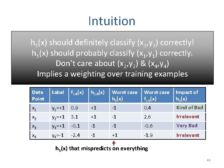
Intuition Aggregate Scoring Function: classify (x , y ) correctly! h 5(x) should definitely 3 3 = f 1: 4(x)+ 0. 5*h 5(x)classify (x 1, y 1) correctly. h 5 f(x) should probably 1: 5(x) care about (x 2 Suppose , y 2) & (x , y 4) Aggregate. Don’t Classifier: a 4= 0. 5 5 Implies a weighting over training examples h 1: 5(x) = sign(f 1: 5(x)) Data Point Label f 1: 4(x) h 1: 4(x) Worst case h 5(x) Worst case f 1: 5(x) Impact of h 5(x) x 1 y 1=+1 0. 9 +1 -1 0. 4 Kind of Bad x 2 y 2=+1 3. 1 +1 -1 2. 6 Irrelevant x 3 y 3=+1 -0. 1 -1 -1 -0. 6 Very Bad x 4 y 4=-1 -2. 4 -1 +1 -1. 9 Irrelevant h 5(x) that mispredicts on everything 44

Intuition Aggregate Scoring Function: f 1: 4(x) = 0. 1*h 1(x) + 1. 5*h 2(x) + 0. 4*h 3(x) + 1. 1*h 4(x) Aggregate Classifier: h 1: 4(x) = sign(f 1: 4(x)) Data Point Label f 1: 4(x) h 1: 4(x) Desired D 5 x 1 y 1=+1 0. 9 +1 Medium x 2 y 2=+1 3. 1 +1 Low x 3 y 3=+1 -0. 1 -1 High x 4 y 4=-1 -2. 4 -1 Low 45

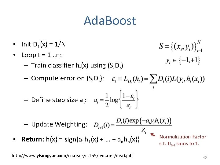
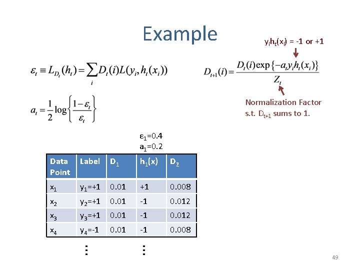
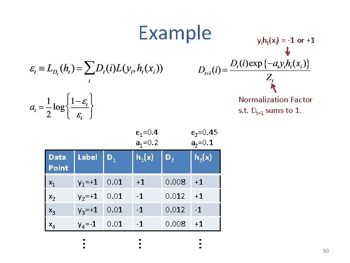
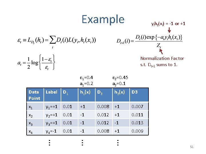
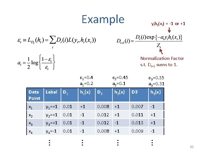
Ada. Boost • Init D 1(x) = 1/N • Loop t = 1…n: – Train classifier ht(x) using (S, Dt) – Compute error on (S, Dt): – Define step size at: – Update Weighting: • Return: h(x) = sign(a 1 h 1(x) + … + anhn(x)) http: //www. yisongyue. com/courses/cs 155/lectures/msri. pdf Normalization Factor s. t. Dt+1 sums to 1. 46

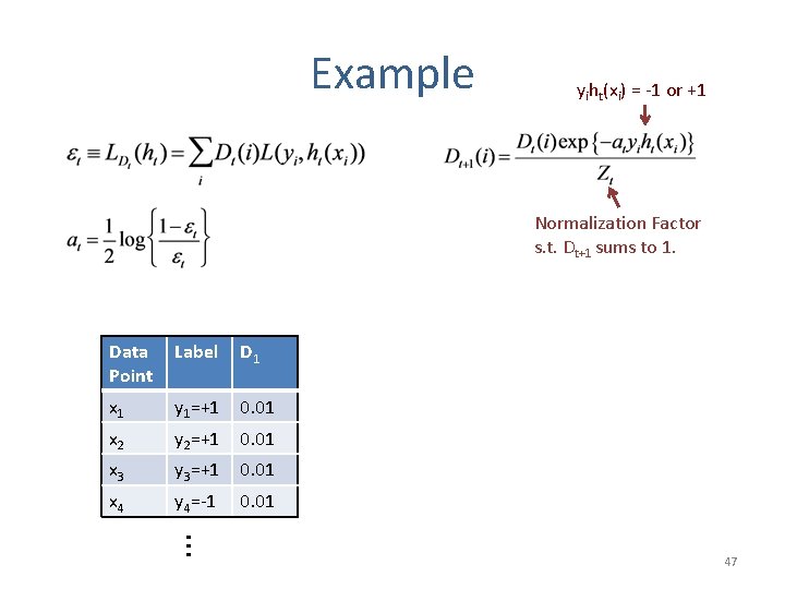
Example yiht(xi) = -1 or +1 Normalization Factor s. t. Dt+1 sums to 1. Data Point Label D 1 x 1 y 1=+1 0. 01 x 2 y 2=+1 0. 01 x 3 y 3=+1 0. 01 x 4 y 4=-1 0. 01 … 47

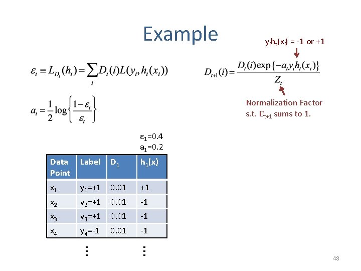
Example yiht(xi) = -1 or +1 Normalization Factor s. t. Dt+1 sums to 1. ε 1=0. 4 a 1=0. 2 Data Point Label D 1 h 1(x) x 1 y 1=+1 0. 01 +1 x 2 y 2=+1 0. 01 -1 x 3 y 3=+1 0. 01 -1 x 4 y 4=-1 0. 01 -1 … … 48

Example yiht(xi) = -1 or +1 Normalization Factor s. t. Dt+1 sums to 1. ε 1=0. 4 a 1=0. 2 Data Point Label D 1 h 1(x) D 2 x 1 y 1=+1 0. 01 +1 0. 008 x 2 y 2=+1 0. 01 -1 0. 012 x 3 y 3=+1 0. 01 -1 0. 012 x 4 y 4=-1 0. 01 -1 0. 008 … … 49

Example yiht(xi) = -1 or +1 Normalization Factor s. t. Dt+1 sums to 1. ε 1=0. 4 a 1=0. 2 ε 2=0. 45 a 2=0. 1 Data Point Label D 1 h 1(x) D 2 h 2(x) x 1 y 1=+1 0. 01 +1 0. 008 +1 x 2 y 2=+1 0. 01 -1 0. 012 +1 x 3 y 3=+1 0. 01 -1 0. 012 -1 x 4 y 4=-1 0. 01 -1 0. 008 +1 … … … 50

Example yiht(xi) = -1 or +1 Normalization Factor s. t. Dt+1 sums to 1. ε 1=0. 4 a 1=0. 2 ε 2=0. 45 a 2=0. 1 Data Point Label D 1 h 1(x) D 2 h 2(x) D 3 x 1 y 1=+1 0. 01 +1 0. 008 +1 0. 007 x 2 y 2=+1 0. 01 -1 0. 012 +1 0. 011 x 3 y 3=+1 0. 01 -1 0. 012 -1 0. 013 x 4 y 4=-1 0. 01 -1 0. 008 +1 0. 009 … … … 51

Example yiht(xi) = -1 or +1 Normalization Factor s. t. Dt+1 sums to 1. ε 1=0. 4 a 1=0. 2 ε 2=0. 45 a 2=0. 1 ε 3=0. 35 a 3=0. 31 Data Point Label D 1 h 1(x) D 2 h 2(x) D 3 h 3(x) x 1 y 1=+1 0. 01 +1 0. 008 +1 0. 007 -1 x 2 y 2=+1 0. 01 -1 0. 012 +1 0. 011 +1 x 3 y 3=+1 0. 01 -1 0. 012 -1 0. 013 +1 x 4 y 4=-1 0. 01 -1 0. 008 +1 0. 009 -1 … … 52

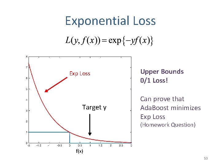
Exponential Loss Exp Loss Target y Upper Bounds 0/1 Loss! Can prove that Ada. Boost minimizes Exp Loss (Homework Question) f(x) 53

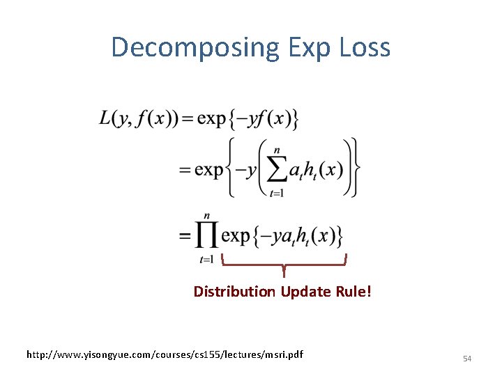
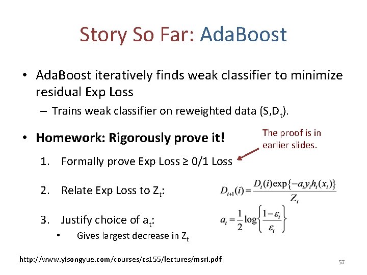
Decomposing Exp Loss Distribution Update Rule! http: //www. yisongyue. com/courses/cs 155/lectures/msri. pdf 54

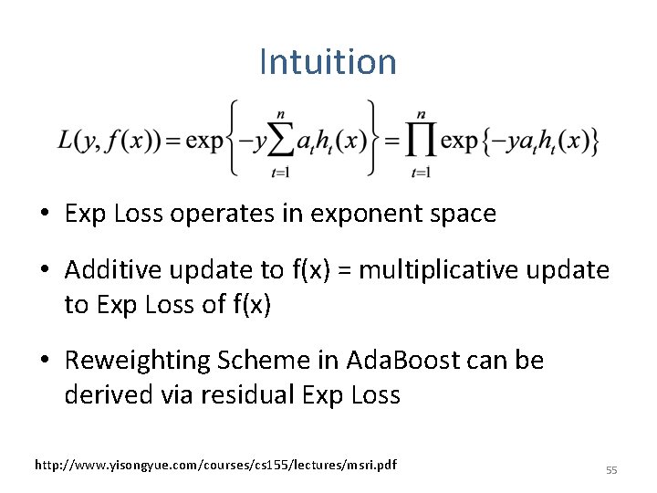
Intuition • Exp Loss operates in exponent space • Additive update to f(x) = multiplicative update to Exp Loss of f(x) • Reweighting Scheme in Ada. Boost can be derived via residual Exp Loss http: //www. yisongyue. com/courses/cs 155/lectures/msri. pdf 55

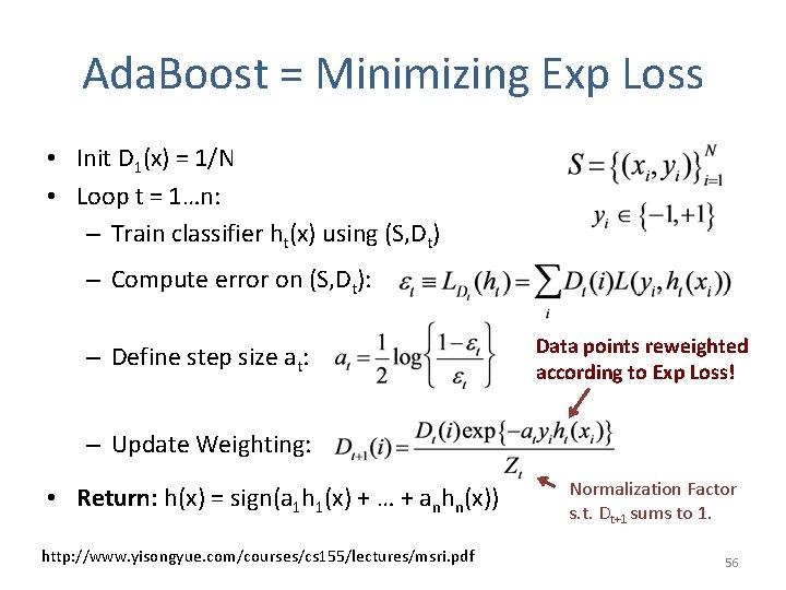
Ada. Boost = Minimizing Exp Loss • Init D 1(x) = 1/N • Loop t = 1…n: – Train classifier ht(x) using (S, Dt) – Compute error on (S, Dt): – Define step size at: Data points reweighted according to Exp Loss! – Update Weighting: • Return: h(x) = sign(a 1 h 1(x) + … + anhn(x)) http: //www. yisongyue. com/courses/cs 155/lectures/msri. pdf Normalization Factor s. t. Dt+1 sums to 1. 56

Story So Far: Ada. Boost • Ada. Boost iteratively finds weak classifier to minimize residual Exp Loss – Trains weak classifier on reweighted data (S, Dt). • Homework: Rigorously prove it! The proof is in earlier slides. 1. Formally prove Exp Loss ≥ 0/1 Loss 2. Relate Exp Loss to Zt: 3. Justify choice of at: • Gives largest decrease in Zt http: //www. yisongyue. com/courses/cs 155/lectures/msri. pdf 57

Recap: Ada. Boost • Gradient Descent in Function Space – Space of weak classifiers • Final model = linear combination of weak classifiers – h(x) = sign(a 1 h 1(x) + … + anhn(x)) – I. e. , a point in Function Space • Iteratively creates new training sets via reweighting – Trains weak classifier on reweighted training set – Derived via minimizing residual Exp Loss 58

Ensemble Selection 59

Recall: Bias-Variance Decomposition • For squared error: Variance Term Bias Term “Average prediction on x” 60

Ensemble Methods • Combine base models to improve performance • Bagging: averages high variance, low bias models – Reduces variance – Indirectly deals with bias via low bias base models • Boosting: carefully combines simple models – Reduces bias – Indirectly deals with variance via low variance base models • Can we get best of both worlds? 61

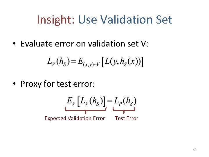
Insight: Use Validation Set • Evaluate error on validation set V: • Proxy for test error: Expected Validation Error Test Error 62

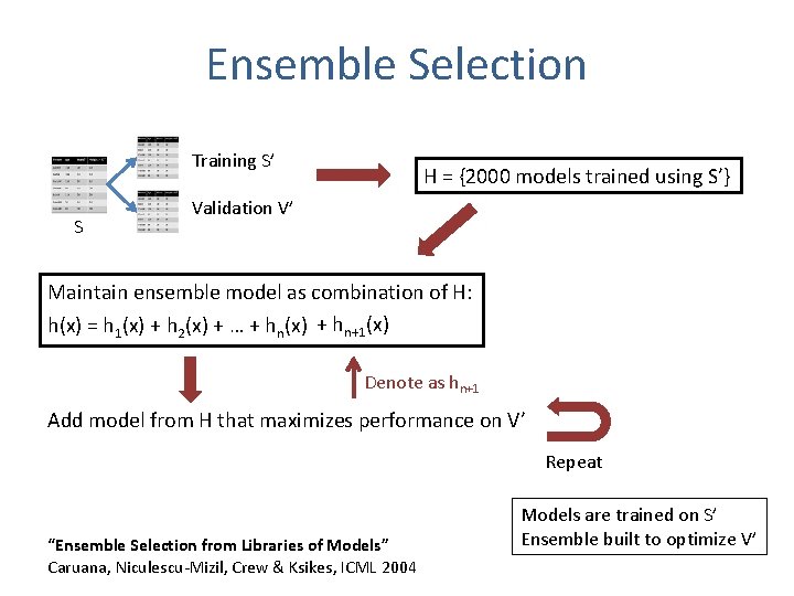
Ensemble Selection Training S’ S H = {2000 models trained using S’} Validation V’ Maintain ensemble model as combination of H: h(x) = h 1(x) + h 2(x) + … + hn(x) + hn+1(x) Denote as hn+1 Add model from H that maximizes performance on V’ Repeat “Ensemble Selection from Libraries of Models” Caruana, Niculescu-Mizil, Crew & Ksikes, ICML 2004 Models are trained on S’ Ensemble built to optimize V’

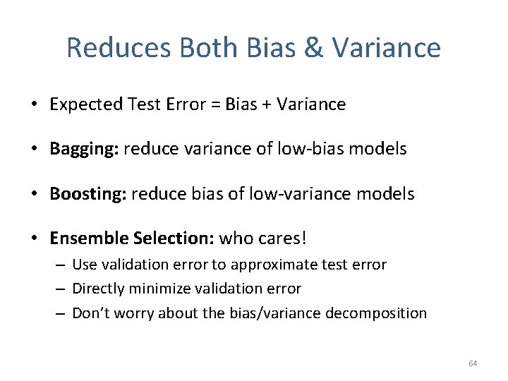
Reduces Both Bias & Variance • Expected Test Error = Bias + Variance • Bagging: reduce variance of low-bias models • Boosting: reduce bias of low-variance models • Ensemble Selection: who cares! – Use validation error to approximate test error – Directly minimize validation error – Don’t worry about the bias/variance decomposition 64

What’s the Catch? • Relies heavily on validation set – Bagging & Boosting: uses training set to select next model – Ensemble Selection: uses validation set to select next model • Requires validation set be sufficiently large • In practice: implies smaller training sets – Training & validation = partitioning of finite data • Often works very well in practice 65

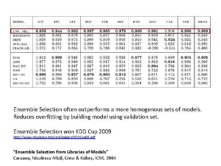
Ensemble Selection often outperforms a more homogenous sets of models. Reduces overfitting by building model using validation set. Ensemble Selection won KDD Cup 2009 http: //www. niculescu-mizil. org/papers/KDDCup 09. pdf “Ensemble Selection from Libraries of Models” Caruana, Niculescu-Mizil, Crew & Ksikes, ICML 2004

References & Further Reading “An Empirical Comparison of Voting Classification Algorithms: Bagging, Boosting, and Variants” Bauer & Kohavi, Machine Learning, 36, 105– 139 (1999) “Bagging Predictors” Leo Breiman, Tech Report #421, UC Berkeley, 1994, http: //statistics. berkeley. edu/sites/default/files/tech-reports/421. pdf “An Empirical Comparison of Supervised Learning Algorithms” Caruana & Niculescu-Mizil, ICML 2006 “An Empirical Evaluation of Supervised Learning in High Dimensions” Caruana, Karampatziakis & Yessenalina, ICML 2008 “Ensemble Methods in Machine Learning” Thomas Dietterich, Multiple Classifier Systems, 2000 “Ensemble Selection from Libraries of Models” Caruana, Niculescu-Mizil, Crew & Ksikes, ICML 2004 “Getting the Most Out of Ensemble Selection” Caruana, Munson, & Niculescu-Mizil, ICDM 2006 “Explaining Ada. Boost” Rob Schapire, https: //www. cs. princeton. edu/~schapire/papers/explaining-adaboost. pdf “Greedy Function Approximation: A Gradient Boosting Machine”, Jerome Friedman, 2001, http: //statweb. stanford. edu/~jhf/ftp/trebst. pdf “Random Forests – Random Features” Leo Breiman, Tech Report #567, UC Berkeley, 1999, “Structured Random Forests for Fast Edge Detection” Dollár & Zitnick, ICCV 2013 “ABC-Boost: Adaptive Base Class Boost for Multi-class Classification” Ping Li, ICML 2009 “Additive Groves of Regression Trees” Sorokina, Caruana & Riedewald, ECML 2007, http: //additivegroves. net/ “Winning the KDD Cup Orange Challenge with Ensemble Selection”, Niculescu-Mizil et al. , KDD 2009 “Lessons from the Netflix Prize Challenge” Bell & Koren, SIGKDD Exporations 9(2), 75— 79, 2007

Next Week • Office Hours Today: – Finding group members for mini-project • Next Week: – Extensions of Decision Trees – Learning Reductions • How to combine binary classifiers to solve more complicated prediction tasks 68