Machine Learning Crash Course Photo CMU Machine Learning

Machine Learning Crash Course Photo: CMU Machine Learning Department protests G 20 Computer Vision James Hays Slides: Isabelle Guyon, Erik Sudderth, Mark Johnson, Derek Hoiem

Robert Borowicz

Bao Vu

Creston Bunch

Pranathi Tupakula

Murali Raghu Babu Balusu

Sandhya Sridhar

M S Suraj

Machine Learning Crash Course Photo: CMU Machine Learning Department protests G 20 Computer Vision James Hays Slides: Isabelle Guyon, Erik Sudderth, Mark Johnson, Derek Hoiem

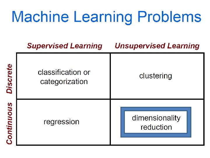
Dimensionality Reduction • PCA, ICA, LLE, Isomap • PCA is the most important technique to know. It takes advantage of correlations in data dimensions to produce the best possible lower dimensional representation based on linear projections (minimizes reconstruction error). • PCA should be used for dimensionality reduction, not for discovering patterns or making predictions. Don't try to assign semantic meaning to the bases.

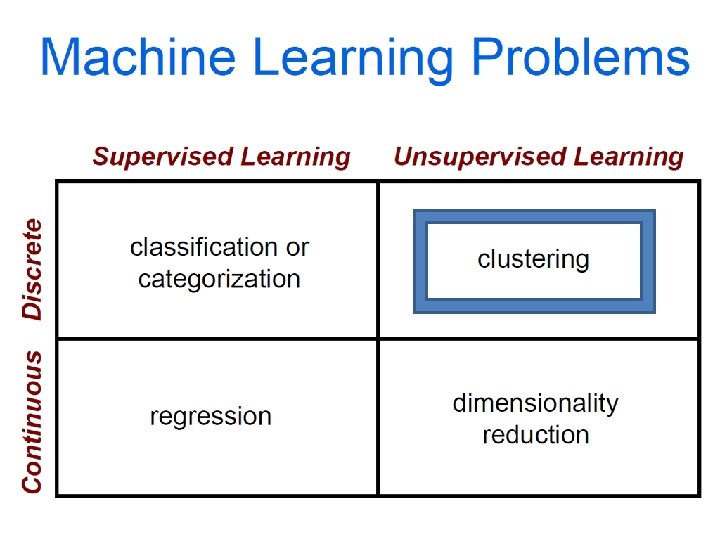
How do we cluster? • K-means – Iteratively re-assign points to the nearest cluster center • Agglomerative clustering – Start with each point as its own cluster and iteratively merge the closest clusters • Mean-shift clustering – Estimate modes of pdf • Spectral clustering – Split the nodes in a graph based on assigned links with similarity weights

Clustering for Summarization Goal: cluster to minimize variance in data given clusters – Preserve information Cluster center Data Whether xj is assigned to ci Slide: Derek Hoiem

K-means algorithm 1. Randomly select K centers 2. Assign each point to nearest center 3. Compute new center (mean) for each cluster Illustration: http: //en. wikipedia. org/wiki/K-means_clustering

K-means algorithm 1. Randomly select K centers 2. Assign each point to nearest center 3. Compute new center (mean) for each cluster Illustration: http: //en. wikipedia. org/wiki/K-means_clustering Back to 2

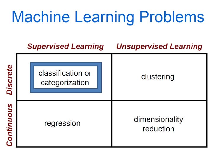
The machine learning framework • Apply a prediction function to a feature representation of the image to get the desired output: f( f( f( ) = “apple” ) = “tomato” ) = “cow” Slide credit: L. Lazebnik

The machine learning framework y = f(x) output prediction function Image feature • Training: given a training set of labeled examples {(x 1, y 1), …, (x. N, y. N)}, estimate the prediction function f by minimizing the prediction error on the training set • Testing: apply f to a never before seen test example x and output the predicted value y = f(x) Slide credit: L. Lazebnik

Learning a classifier Given some set of features with corresponding labels, learn a function to predict the labels from the features x x o x x x o o o x 2 x 1 o x x x

Steps Training Labels Training Images Image Features Training Learned model Prediction Testing Image Features Test Image Slide credit: D. Hoiem and L. Lazebnik

Features • Raw pixels • Histograms • GIST descriptors • … Slide credit: L. Lazebnik

One way to think about it… • Training labels dictate that two examples are the same or different, in some sense • Features and distance measures define visual similarity • Classifiers try to learn weights or parameters for features and distance measures so that visual similarity predicts label similarity

Many classifiers to choose from • • • SVM Neural networks Which is the best one? Naïve Bayesian network Logistic regression Randomized Forests Boosted Decision Trees K-nearest neighbor RBMs Deep Convolutional Network Etc.

Claim: The decision to use machine learning is more important than the choice of a particular learning method. *Deep learning seems to be an exception to this, at the moment, probably because it is learning the feature representation.

Classifiers: Nearest neighbor Training examples from class 1 Test example Training examples from class 2 f(x) = label of the training example nearest to x • All we need is a distance function for our inputs • No training required! Slide credit: L. Lazebnik

Classifiers: Linear • Find a linear function to separate the classes: f(x) = sgn(w x + b) Slide credit: L. Lazebnik

Recognition task and supervision • Images in the training set must be annotated with the “correct answer” that the model is expected to produce Contains a motorbike Slide credit: L. Lazebnik

Unsupervised “Weakly” supervised Fully supervised Definition depends on task Slide credit: L. Lazebnik

Generalization Training set (labels known) Test set (labels unknown) • How well does a learned model generalize from the data it was trained on to a new test set? Slide credit: L. Lazebnik

Generalization • Components of generalization error – Bias: how much the average model over all training sets differ from the true model? • Error due to inaccurate assumptions/simplifications made by the model. – Variance: how much models estimated from different training sets differ from each other. • Underfitting: model is too “simple” to represent all the relevant class characteristics – High bias (few degrees of freedom) and low variance – High training error and high test error • Overfitting: model is too “complex” and fits irrelevant characteristics (noise) in the data – Low bias (many degrees of freedom) and high variance – Low training error and high test error Slide credit: L. Lazebnik

Bias-Variance Trade-off • Models with too few parameters are inaccurate because of a large bias (not enough flexibility). • Models with too many parameters are inaccurate because of a large variance (too much sensitivity to the sample). Slide credit: D. Hoiem

Bias-Variance Trade-off E(MSE) = noise 2 + bias 2 + variance Unavoidable error Error due to incorrect assumptions Error due to variance of training samples See the following for explanations of bias-variance (also Bishop’s “Neural Networks” book): • http: //www. inf. ed. ac. uk/teaching/courses/mlsc/Notes/Lecture 4/Bias. Variance. pdf Slide credit: D. Hoiem

Bias-variance tradeoff Overfitting Error Underfitting Test error Training error High Bias Low Variance Complexity Low Bias High Variance Slide credit: D. Hoiem

Bias-variance tradeoff Test Error Few training examples High Bias Low Variance Many training examples Complexity Low Bias High Variance Slide credit: D. Hoiem

Effect of Training Size Error Fixed prediction model Testing Generalization Error Training Number of Training Examples Slide credit: D. Hoiem

Remember… • No classifier is inherently better than any other: you need to make assumptions to generalize • Three kinds of error – Inherent: unavoidable – Bias: due to over-simplifications – Variance: due to inability to perfectly estimate parameters from limited data Slide credit: D. Hoiem

How to reduce variance? • Choose a simpler classifier • Regularize the parameters • Get more training data Slide credit: D. Hoiem

Very brief tour of some classifiers • • • K-nearest neighbor SVM Boosted Decision Trees Neural networks Naïve Bayesian network Logistic regression Randomized Forests RBMs Etc.

Generative vs. Discriminative Classifiers Generative Models Discriminative Models • Represent both the data and • Learn to directly predict the labels from the data • Often, makes use of • Often, assume a simple conditional independence boundary (e. g. , linear) and priors • Examples – Logistic regression – Naïve Bayes classifier – Bayesian network – SVM – Boosted decision trees • Models of data may apply to • Often easier to predict a label from the data than to future prediction problems model the data Slide credit: D. Hoiem

Classification • Assign input vector to one of two or more classes • Any decision rule divides input space into decision regions separated by decision boundaries Slide credit: L. Lazebnik

Nearest Neighbor Classifier • Assign label of nearest training data point to each test data point from Duda et al. Voronoi partitioning of feature space for two-category 2 D and 3 D data Source: D. Lowe

K-nearest neighbor x x o x + o o x 2 x 1 x o+ x x x

1 -nearest neighbor x x o x + o o x 2 x 1 x o+ x x x

3 -nearest neighbor x x o x + o o x 2 x 1 x o+ x x x

5 -nearest neighbor x x o x + o o x 2 x 1 x o+ x x x

Using K-NN • Simple, a good one to try first • With infinite examples, 1 -NN provably has error that is at most twice Bayes optimal error

Classifiers: Linear SVM x x x o o x x x o x 2 x 1 • Find a linear function to separate the classes: f(x) = sgn(w x + b)

Classifiers: Linear SVM x x x o o x x x o x 2 x 1 • Find a linear function to separate the classes: f(x) = sgn(w x + b)

Classifiers: Linear SVM x x x o o o x x x o x 2 x 1 • Find a linear function to separate the classes: f(x) = sgn(w x + b)

What about multi-class SVMs? • Unfortunately, there is no “definitive” multiclass SVM formulation • In practice, we have to obtain a multi-class SVM by combining multiple two-class SVMs • One vs. others • Traning: learn an SVM for each class vs. the others • Testing: apply each SVM to test example and assign to it the class of the SVM that returns the highest decision value • One vs. one • Training: learn an SVM for each pair of classes • Testing: each learned SVM “votes” for a class to assign to the test example Slide credit: L. Lazebnik

SVMs: Pros and cons • Pros • Many publicly available SVM packages: http: //www. kernel-machines. org/software • Kernel-based framework is very powerful, flexible • SVMs work very well in practice, even with very small training sample sizes • Cons • No “direct” multi-class SVM, must combine two-class SVMs • Computation, memory – During training time, must compute matrix of kernel values for every pair of examples – Learning can take a very long time for large-scale problems

What to remember about classifiers • No free lunch: machine learning algorithms are tools, not dogmas • Try simple classifiers first • Better to have smart features and simple classifiers than simple features and smart classifiers • Use increasingly powerful classifiers with more training data (bias-variance tradeoff) Slide credit: D. Hoiem

Making decisions about data • 3 important design decisions: 1) What data do I use? 2) How do I represent my data (what feature)? 3) What classifier / regressor / machine learning tool do I use? • These are in decreasing order of importance • Deep learning addresses 2 and 3 simultaneously (and blurs the boundary between them). • You can take the representation from deep learning and use it with any classifier.