Machine Learning BE Computer 2015 PAT A Y
 A. Y. 2018 -19 SEM-II Prepared by Mr.")
Machine Learning (BE Computer 2015 PAT) A. Y. 2018 -19 SEM-II Prepared by Mr. Dhomse G. P.

Unit-2 Feature Selection Syllabus • Scikit- learn Dataset, Creating training and test sets, 1 hr • managing categorical data, 1 hr • Managing missing features, 1 hr • Data scaling and normalization, 1 hr • Feature selection and Filtering, 1 hr • Principle Component Analysis(PCA)-non negative matrix factorization, 1 hr • Sparse PCA, Kernel PCA. 1 hr • Atom Extraction and Dictionary Learning. 1 hr

scikit-learn toy datasets • scikit-learn provides some built-in datasets that can be used for testing purposes. • They're all available in the package sklearn. datasets and have a common structure: the data instance variable contains the whole input set X while target contains the labels for classification or target values for regression.

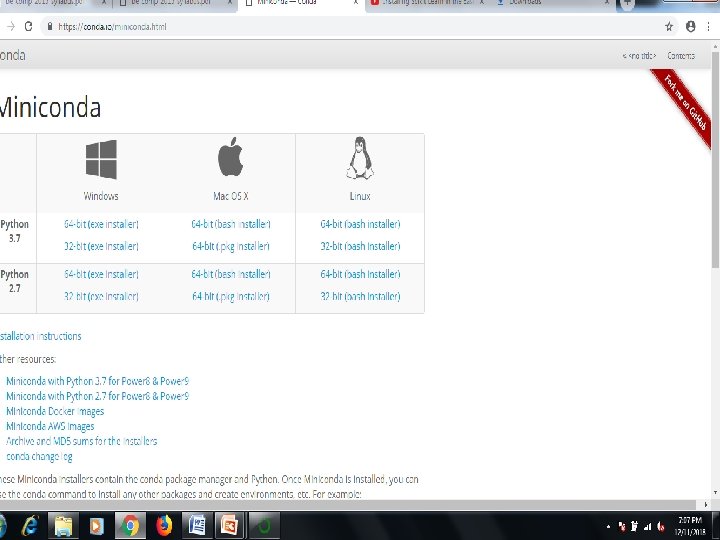
Step by Step Scikit • Installing the Python and Sci. Py platform. -Download Miniconda • Loading the dataset. • Summarizing the dataset. • Visualizing the dataset. • Evaluating some algorithms. • Making some predictions.
 command prompt Enter Following Command")
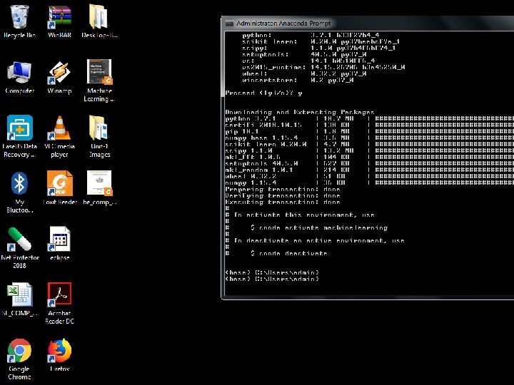
• • • Open Anaconda 3 (32 bit) command prompt Enter Following Command One by One Open Site- https: //conda. io/docs/using/envs. html Anaconda Prompt for the following steps. To create an environment: conda create --name myenv NOTE: Replace myenv with the environment name. I replace myenv with machineleaning scikit-learn When conda asks you to proceed, type y: proceed ([y]/n)? After finish of installation use the above command $ conda activate machinelearning

• This creates the myenv environment in /envs/. This environment uses the same version of Python that you are currently using, because you did not specify a version. To create an environment with a specific version of Python: • $ conda create -n myenv python=3. 4 • To create an environment with a specific package: • conda create -n myenv scipy To create an environment with a specific version of a package: $ conda create -n myenv scipy=0. 15. 0 • Now type Python to open the python prompt >>>
, we")
• For example, considering the Boston house pricing dataset (used for regression), we have: • Load and return the boston house-prices dataset (regression). • Samples total 506 • Dimensionality 13 • Features real, positive • Targets real 5. - 50.

• Now type Python to open the python prompt >>> Now type following code on python prompt from sklearn. datasets import load_boston >>> boston = load_boston() >>> X = boston. data >>> Y = boston. target >>> X. shape (506, 13) >>> Y. shape

Getting started in scikit-learn with the famous iris dataset • https: //github. com/justmarkham/scikit-learnvideos/blob/master/03_getting_started_with _iris. ipynb • What is the famous iris dataset, and how does it relate to machine learning? • How do we load the iris dataset into scikit-learn? • How do we describe a dataset using machine learning terminology? • What are scikit-learn's four key requirements for working with data?
 Measurements:")
iris flower 50 samples of 3 different species of iris (150 samples total) Measurements: sepal length, sepal width, petal length, petal width

• # import load_iris function from datasets module >>> from sklearn. datasets import load_iris # save "bunch" object containing iris dataset and its attributes iris = load_iris() type(iris) >>> sklearn. datasets. base. Bunch # print the iris data >>> print(iris. data) See the Output Matrix contain- • Each row is an observation (also known as: sample, example, instance, record) • Each column is a feature (also known as: predictor, attribute, independent variable, input, regressor, covariate)
![• • • [[ 5. 1 3. 5 1. 4 0. 2] [](http://slidetodoc.com/presentation_image_h2/fe2e1264f85f3232a7fc9e0ef46dcf35/image-15.jpg "• • • [[ 5. 1 3. 5 1. 4 0. 2] [")
• • • [[ 5. 1 3. 5 1. 4 0. 2] [ 4. 9 3. 1. 4 0. 2] [ 4. 7 3. 2 1. 3 0. 2] [ 4. 6 3. 1 1. 5 0. 2] [ 5. 3. 6 1. 4 0. 2] [ 5. 4 3. 9 1. 7 0. 4] [ 4. 6 3. 4 1. 4 0. 3] [ 5. 3. 4 1. 5 0. 2] [ 4. 4 2. 9 1. 4 0. 2] [ 4. 9 3. 1 1. 5 0. 1]…. .
 O/P-")
• # print the names of the four features >>> print(iris. feature_names) O/P- ['sepal length (cm)', 'sepal width (cm)', 'petal length (cm)', 'petal width (cm)'] # print integers representing the species of each observation >>> print(iris. target) [0 0 0 0 0 0 0 0000000000111111111111111222222222222222 2 2]

• # print the encoding scheme for species: 0 = setosa, 1 = versicolor, 2 = virginica >>> print(iris. target_names) O/P- ['setosa' 'versicolor' 'virginica'] • Each value we are predicting is the response (also known as: target, outcome, label, dependent variable) • Classification is supervised learning in which the response is categorical • Regression is supervised learning in which the response is ordered and continuous

• Requirements for working with data in scikitlearn • Features and response are separate objects • Features and response should be numeric • Features and response should be Num. Py arrays • Features and response should have specific shapes
)")
• # check the types of the features and response >>> print(type(iris. data)) >>> print(type(iris. target)) O/P- <type 'numpy. ndarray'> # check the shape of the features (first dimension = number of observations, second dimensions = number of features) >>> print(iris. data. shape) O/P- (150 L, 4 L)

• # check the shape of the response (single dimension matching the number of observations) >>> print(iris. target. shape) O/P- (150 L, ) # store feature matrix in "X“ >>> X = iris. data # store response vector in "y" >>> y = iris. target

Basics • Numpy –Numerical Python is: -extension package to Python for multidimensional arrays • closer to hardware (efficiency) • ndarray, a fast and space-efficient multidimensional array providing vectorized arithmetic operation • An ndarray is a generic multidimensional container for homogeneous data; that is, all of the elements must be the same type. • Every array has a shape, a tuple indicating the size of each dimension, and a dtype, an object describing the data type of the array:
![In [13]: data 1 = [6, 7. 5, 8, 0, 1] In [14]: arr](http://slidetodoc.com/presentation_image_h2/fe2e1264f85f3232a7fc9e0ef46dcf35/image-22.jpg "In [13]: data 1 = [6, 7. 5, 8, 0, 1] In [14]: arr")
In [13]: data 1 = [6, 7. 5, 8, 0, 1] In [14]: arr 1 = np. array(data 1) In [15]: arr 1 Out[15]: array([ 6. , 7. 5, 8. , 0. , 1. ]) In [16]: data. dtype Out[16]: dtype(‘int 64') Convert input data (list, tuple, array, or other sequence type) to an ndarray either by inferring a dtype or explicitly specifying a dtype. Copies the input data by default.

Creating training and test sets

• When a dataset is large enough, it's a good practice to split it into training and test sets; the former to be used for training the model and the latter to test its performances. • There are two main rules in performing such an operation: • Both datasets must reflect the original distribution • The original dataset must be randomly shuffled before the split phase in order to avoid a correlation between consequent elements

>>> import numpy as np >>> from sklearn. model_selection import train_test_split >>> X, y = np. arange(10). reshape((5, 2)), range(5) >>> X O/P-array ([[0, 1], [2, 3], [4, 5], [6, 7], [8, 9]]) >>> list(y) o/p- [0, 1, 2, 3, 4]
")
>>> X_train, X_test, y_train, y_test = train_test_split(. . . X, y, test_size=0. 25, random_state=100) >>> X_train O/P- array ([ [6, 7], [8, 9], [0, 1]]) >>> y_train [3, 4, 0] >>> X_test array([[2, 3], [4, 5]]) >>> y_test [1, 2]
 allows specifying the percentage of")
• The parameter test_size (as well as training_size) allows specifying the percentage of elements to put into the test/training set. In this case, the ratio is 75 percent for training and 25 percent for the test phase. • Another important parameter is random_state which can accept a Num. Py Random. State generator or an integer seed. • In many cases, it's important to provide reproducibility for the experiments,

Managing categorical data • Not all data has numerical values. Here are examples of categorical data: • The blood type of a person: A, B, AB or O. • The state that a resident of the United States lives in. • ["male", "female"], • ["from Europe", "from US", "from Asia"], • ["uses Firefox", "uses Chrome", "uses Saf ari", "uses Internet Explorer"].

• Such features can be efficiently coded as integers, for • • instance ["male", "from US", "uses Internet Ex plorer"] could be expressed as [0, 1, 3] while ["female", "from Asia", "uses Chrome"] would be [1, 2, 1]. Before Start Categorical data Install pandas to run python based pandas program $ pip install pandas

Basic- Pandas

• To convert categorical features to such integer codes, we can use the Ordinal. Encoder • This estimator transforms each categorical feature to one new feature of integers (0 to n_categories - 1): >>> import numpy as np >>> X = np. random. uniform(0. 0, 1. 0, size=(10, 2)) >>> Y = np. random. choice(('Male', 'Female'), size=(10)) >>> X[0] array([ 0. 8236887 , 0. 11975305]) >>> Y[0]
 Return a random floating point number N such")
Code Explanation • random. uniform(a, b) Return a random floating point number N such that a <= N <= b for a <= b and b <= N <= a for b < a. • random. choice is used to replace the categorial value into other integer or float number • Label. Encoder class- it used Encode labels with value between 0 and n_classes-1. Label. Encoder can be used to normalize labels.

• The first option is to use the Label. Encoder class, which adopts a dictionary-oriented approach, associating to each category label a progressive integer number, that is an index of an instance array called classes_: from sklearn. preprocessing import Label. Encoder >>> le = Label. Encoder() >>> yt = le. fit_transform(Y) >>> print(yt) [0 0 0 1 1 0 0 1]

• Label. Encoder can be used to normalize labels. • It can also be used to transform non-numerical labels (as long as they are hashable and comparable) to numerical labels. • Fit Transform Fit label encoder and return encoded labels • transform replaces the missing values with a number. • So by fit the imputer calculates the means of columns from some data, and by transform it applies those means to some data (which is just replacing missing values with the means). If both these data are the same (i. e. the data for calculating the means and the data that means are applied to) you can use fit_transform which is basically a fit followed by a transform.
![Exampleimp = Imputer() # calculating the means imp. fit([[1, 3], [np. nan, 2], [8,](http://slidetodoc.com/presentation_image_h2/fe2e1264f85f3232a7fc9e0ef46dcf35/image-35.jpg "Exampleimp = Imputer() # calculating the means imp. fit([[1, 3], [np. nan, 2], [8,")
Exampleimp = Imputer() # calculating the means imp. fit([[1, 3], [np. nan, 2], [8, 5. 5]]) Now the imputer have learned to use a mean (1+8)/2 = 4. 5 for the first column and mean (2+3+5. 5)/3 = 3. 5 for the second column when it gets applied to a twocolumn data: X = [[np. nan, 11], [4, np. nan], [8, 2], [np. nan, 1]] print(imp. transform(X)) we get
![Coding Continue from side 33 >>> le. classes_ array(['Female', 'Male'], dtype=‘<U 6') The inverse](http://slidetodoc.com/presentation_image_h2/fe2e1264f85f3232a7fc9e0ef46dcf35/image-36.jpg "Coding Continue from side 33 >>> le. classes_ array(['Female', 'Male'], dtype=‘<U 6') The inverse")
Coding Continue from side 33 >>> le. classes_ array(['Female', 'Male'], dtype=‘<U 6') The inverse transformation can be obtained in this simple way: >>> le. inverse_transform([1, 0]) it has a drawback: all labels are turned into sequential numbers. A classifier which works with real values will then consider similar numbers according to their distance, without any concern for semantics. For this reason, it's often preferable to use so-called one-hot encoding, which binarizes the data. For labels, it can be achieved using the Label. Binarizer class:
 >>> Yb =")
from sklearn. preprocessing import Label. Binarizer >>> lb = Label. Binarizer() >>> Yb = lb. fit_transform(Y) >>>print(Yb) array([[0], [0] [0] [1] to convert categorical features to features that can be used with scikit-learn estimators is to use a one-of-K, also known as one-hot or dummy encoding. This type of encoding can be obtained with the One. Hot. Encoder, which transforms each categorical feature with n_categories possible values into n_categories binary features, with one of them 1, and all others 0.
![>>> lb. inverse_transform(Yb) array(['Female', 'Female', 'Male', ], dtype=‘<U 6') Now predict the Binary Feature](http://slidetodoc.com/presentation_image_h2/fe2e1264f85f3232a7fc9e0ef46dcf35/image-38.jpg ">>> lb. inverse_transform(Yb) array(['Female', 'Female', 'Male', ], dtype=‘<U 6') Now predict the Binary Feature")
>>> lb. inverse_transform(Yb) array(['Female', 'Female', 'Male', ], dtype=‘<U 6') Now predict the Binary Feature 1 is it male or female? ? ? >>> import numpy as np >>> Y = lb. fit_transform(Y) array ([[0, 1, 0, 0, 0], [0, 0, 0, 1, 0], [1, 0, 0]]) >>> Yp = model. predict(X[0]) array([[0. 002, 0. 991, 0. 005, 0. 001]]) >>> Ypr = np. round(Yp) ([[ 0. , 1. , 0. ]]) >>> lb. inverse_transform(Ypr) array(['Female'], dtype=‘’<U 6')

to categorical features can be adopted when they're structured like a list of dictionaries • data = [{ 'feature_1': 10. 0, 'feature_2': 15. 0 }, { 'feature_1': -5. 0, 'feature_3': 22. 0 }, { 'feature_3': -2. 0, 'feature_4': 10. 0 } ] classes Dict. Vectorizer and Feature. Hasher; they both produce sparse matrices of real numbers that can be fed into any machine learning model. Dict. Vectorizer vectorizes string-valued features using a hash table. Feature. Hasher-This class turns sequences of symbolic feature names (strings) into scipy. sparse matrices, using a hash function to compute the matrix column corresponding to a name. The hash function employed is the signed 32 -bit version of Murmurhash 3.
 >>>")
from sklearn. feature_extraction import Dict. Vectorizer, Feature. Hasher >>> dv = Dict. Vectorizer() >>> Y_dict = dv. fit_transform(data) >>> Y_dict. todense() #dence means Matrix Format matrix([[ 10. , 15. , 0. ], [-5. , 0. , 22. , 0. ], [0. , -2. , 10. ]]) >>> dv. vocabulary_ {'feature_1': 0, 'feature_2': 1, 'feature_3': 2, 'feature_4': 3} #index , value >>> fh = Feature. Hasher() >>> Y_hashed = fh. fit_transform(data) >>> Y_hashed. todense() matrix([[0. , 0. , . . . , 0. ], [0. , . . . , 0. ]]) • toarray returns an ndarray; todense returns a matrix. If you want a matrix, use todense; otherwise, use toarray .

One. Hot. Encoder • The input to this transformer should be an array-like of integers or strings, denoting the values taken on by categorical (discrete) features. The features are encoded using a one-hot (aka ‘one-of-K’ or ‘dummy’) encoding scheme. This creates a binary column for each category and returns a sparse matrix or dense array. • By default, the encoder derives the categories based on the unique values in each feature. • The One. Hot. Encoder previously assumed that the input features take on values in the range [0, max(values)).
![from sklearn. preprocessing import One. Hot. Encoder >>> data = [ [0, 10], [1,](http://slidetodoc.com/presentation_image_h2/fe2e1264f85f3232a7fc9e0ef46dcf35/image-42.jpg "from sklearn. preprocessing import One. Hot. Encoder >>> data = [ [0, 10], [1,")
from sklearn. preprocessing import One. Hot. Encoder >>> data = [ [0, 10], [1, 11], [1, 8], [0, 12], [0, 15]] >>> oh = One. Hot. Encoder(categorical_features=[0]) >>> Y_oh = oh. fit_transform(data 1) • >>> Y_oh. todense() matrix([ [ 1. , 0. , 10. ], [0. , 11. ], [0. , 1. , 8. ], [1. , 0. , 12. ], [1. , 0. , 15. ]]) See the output Dummy value is Added as 0 and 1 in Matrix
 encoding of the categorical")
Summery • sklearn. preprocessing. Ordinal. Encoder performs an ordinal (integer) encoding of the categorical features. • sklearn. feature_extraction. Dict. Vectorizer performs a one -hot encoding of dictionary items (also handles stringvalued features). • sklearn. feature_extraction. Feature. Hasher performs an approximate one-hot encoding of dictionary items or strings. • sklearn. preprocessing. Label. Binarizer binarizes labels in a one-vs-all fashion. • sklearn. preprocessing. Multi. Label. Binarizer transforms between iterable of iterables and a multilabel format, e. g. a (samples x classes) binary matrix indicating the presence of a class label.

Managing missing features • a dataset can contain missing features, so there a few options that can be taken into account: • Removing the whole line- dataset is quite large, the number of missing features is high, and any prediction could be risky. • Creating sub-model to predict those featuresmore difficult because it's necessary to determine a supervised strategy to train a model for each feature and, finally, to predict their value. • Using an automatic strategy to input them according to the other known values-likely to be the best choice.

• the class Imputer, which is responsible for filling the holes using a strategy based on the mean (default choice), median, or frequency (the most frequent entry will be used for all the missing ones). • Already See this topic on PPT NO-33

DATA Scaling & Normalization
 is")
• A generic dataset (we assume here that it is always numerical) is made up of different values which can be drawn from different distributions, having different scales and, sometimes, there also outliers. • it's always preferable to standardize datasets before processing them. A very common problem derives from having a non-zero mean and a variance greater than one. • It's possible to specify if the scaling process must include both mean and standard deviation using the parameters with_mean=True/False and with_std=True/False (by default they're both active).

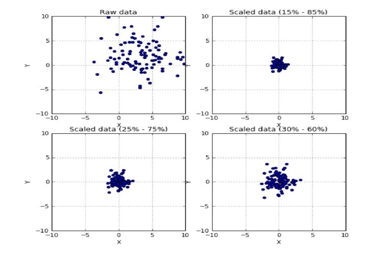
• with a superior control on outliers and the possibility to select a quantile range, there's also the class • This Scaler removes the median and scales the data according to the quantile range (defaults to IQR: Interquartile Range). The IQR is the range between the 1 st quartile (25 th quantile) and the 3 rd quartile (75 th quantile). • Centering and scaling happen independently on each feature by computing the relevant statistics on the samples in the training set. Median and interquartile range are then stored to be used on later data using the transform method. • Standardization of a dataset is a common requirement for many machine learning estimators.
) >>>")
from sklearn. preprocessing import Rubust. Scaler >>> rb 1 = Robust. Scaler(quantile_range=(15, 85)) >>> scaled_data 1 = rb 1. fit_transform(data) >>> rb 1 = Robust. Scaler(quantile_range=(25, 75)) >>> scaled_data 1 = rb 1. fit_transform(data) >>> rb 2 = Robust. Scaler(quantile_range=(30, 60)) >>> scaled_data 2 = rb 2. fit_transform(data)

• scikit-learn also provides a class for persample normalization, Normalizer. • Each sample (i. e. each row of the data matrix) with at least one non zero component is rescaled independently of other samples so that its norm (L 1 or L 2) equals one.
![>>> from sklearn. preprocessing import Normalizer >>> X = [[4, 1, 2, 2], .](http://slidetodoc.com/presentation_image_h2/fe2e1264f85f3232a7fc9e0ef46dcf35/image-52.jpg ">>> from sklearn. preprocessing import Normalizer >>> X = [[4, 1, 2, 2], .")
>>> from sklearn. preprocessing import Normalizer >>> X = [[4, 1, 2, 2], . . . [1, 3, 9, 3], . . . [5, 7, 5, 1]] >>> transformer = Normalizer(). fit(X) # fit does nothing. >>> transformer Normalizer(copy=True, norm=‘L 2') >>> transformer. transform(X) array([[0. 8, 0. 2, 0. 4], [0. 1, 0. 3, 0. 9, 0. 3], [0. 5, 0. 7, 0. 5, 0. 1]])

Feature selection and filtering • An unnormalized dataset with many features contains information proportional to the independence of all features and their variance. Let's consider a small dataset with three features, generated with random Gaussian distributions:

• Even without further analysis, it's obvious that the central line (with the lowest variance) is almost constant and doesn't provide any useful information. • the entropy H(X) is quite small, while the other two variables carry more information. • A variance threshold is, therefore, a useful approach to remove all those elements whose contribution (in terms of variability and so, information) is under a predefined level. • scikit-learn provides the class Variance. Threshold that can easily solve this problem.

• Feature selector that removes all lowvariance features. • This feature selection algorithm looks only at the features (X), not the desired outputs (y), and can thus be used for unsupervised learning. • threshold : float, optional. Features with a training-set variance lower than this threshold will be removed. • remove the features that have the same value in all samples.
![>>> X = [[0, 2, 0, 3], [0, 1, 4, 3], [0, 1, 1,](http://slidetodoc.com/presentation_image_h2/fe2e1264f85f3232a7fc9e0ef46dcf35/image-56.jpg ">>> X = [[0, 2, 0, 3], [0, 1, 4, 3], [0, 1, 1,")
>>> X = [[0, 2, 0, 3], [0, 1, 4, 3], [0, 1, 1, 3]] >>> selector = Variance. Threshold() >>> selector. fit_transform(X) array ([[2, 0], [1, 4], [1, 1]]) in order to select the best features according to specific criteria based on F-tests and pvalues, such as chi-square or ANOVA.

• Examples of feature selection that use the classes Select. KBest (which selects the best K high-score features) and Select. Percentile (which selects only a subset of features belonging to a certain percentile) are shown next. • It's possible to apply them both to regression and classification datasets, being careful to select appropriate score functions: chi 2 Chi-squared stats of non-negative features for classification tasks.

>>> from sklearn. datasets import load_digits >>> from sklearn. feature_selection import Select. KBest, chi 2 >>> X, y = load_digits(return_X_y=True) >>> X. shape (1797, 64) >>> X_new = Select. KBest(chi 2, k=20). fit_transform(X, y) >>> X_new. shape (1797, 20) ********************** >>> from sklearn. datasets import load_digits >>> from sklearn. feature_selection import Select. Percentile, chi 2 >>> X, y = load_digits(return_X_y=True) >>> X. shape (1797, 64) >>> X_new = Select. Percentile(chi 2, percentile=10). fit_transform(X, y) >>> X_new. shape (1797, 7)
 >>> class_data. shape (150 L, 4 L) >>> perc_class =")
>>> class_data = load_iris() >>> class_data. shape (150 L, 4 L) >>> perc_class = Select. Percentile(chi 2, percentile=15) >>> X_p = perc_class. fit_transform(class_data, class_data. target) >>> X_p. shape (150 L, 1 L) >>> perc_class. scores_ array([10. 81782088, 3. 59449902, 116. 16984746, 67. 24482759])
 is a technique used to emphasize")
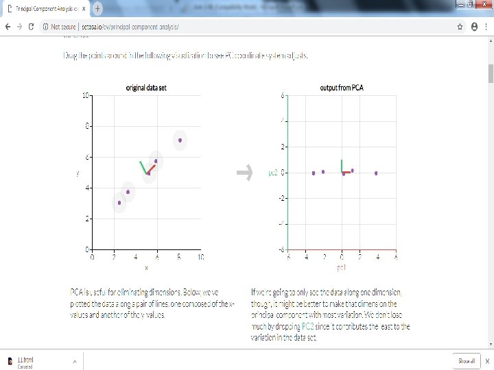
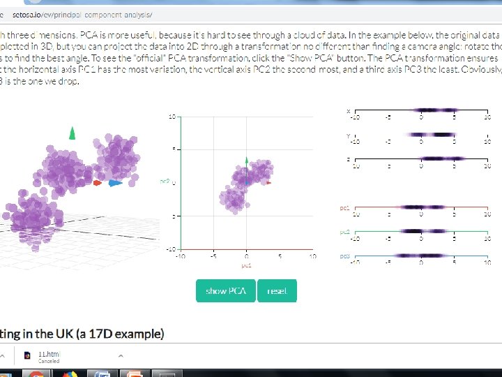
Principal component analysis • Principal component analysis (PCA) is a technique used to emphasize variation and bring out strong patterns in a dataset. It's often used to make data easy to explore and visualize. • First, consider a dataset in only two dimensions, like (height, weight). This dataset can be plotted as points in a plane. But if we want to tease out variation, PCA finds a new coordinate system in which every point has a new (x, y) value. • The axes don't actually mean anything physical; they're combinations of height and weight called "principal components" that are chosen to give one axes lots of variation.


Step by Step PCA • To understand the value of using PCA for data visualization, the first part basic visualization of the IRIS dataset after applying PCA. • The second part uses PCA to speed up a machine learning algorithm (logistic regression) on the MNIST dataset. • matplotlib is a python 2 D plotting library which produces publication quality figures in a variety of hardcopy formats and interactive environments across platforms. matplotlib can be used in Python scripts,

Install to Packages on Anaconda • To install this package with conda run one of the following: for PCA Plot Purpose-2 D etc $ conda install -c conda-forge matplotlib $ conda install -c conda-forge/label/testing/gcc 7 matplotlib $ conda install -c conda-forge/label/broken matplotlib $ conda install -c conda-forge/label/rc matplotlib
 for Data Visualization Source Code- https: //towardsdatascience. com/pca-using-pythonscikit-learn-e 653 f")
Principle Component Analysis (PCA) for Data Visualization Source Code- https: //towardsdatascience. com/pca-using-pythonscikit-learn-e 653 f 8989 e 60 >>>import pandas as pd >>>import numpy as np >>>import matplotlib. pyplot as plt >>>from sklearn. decomposition >>>import PCA from sklearn. preprocessing >>> from sklearn. preprocessing import Standard. Scaler %matplotlib inline

Load Iris Dataset >>>import pandas as pdurl = https: //archive. ics. uci. edu/ml/machinelearning-databases/iris. data # load dataset into Pandas Data. Frame >>>df = pd. read_csv(url, names=['sepal length', 'sepal width', 'petal length', 'petal width', 'target']) >>>df. head()
")
Original Pandas df (features + target)

Standardize the Data • PCA is effected by scale so you need to scale the features in your data before applying PCA. Use Standard. Scaler to help you standardize the dataset’s features onto unit scale (mean = 0 and variance = 1) which is a requirement for the optimal performance of many machine learning algorithms.

>>>from sklearn. preprocessing import Standard. Scalerfeatures = ['sepal length', 'sepal width', 'petal length', 'petal width'] # Separating out the features >>>x = df. loc[: , features]. values # Separating out the target >>>y = df. loc[: , ['target']]. values # Standardizing the features >>>x = Standard. Scaler(). fit_transform(x) >>>pd. Data. Frame(data = x, columns = features). head()
 before and after standardization")
The array x (visualized by a pandas dataframe) before and after standardization

PCA Projection to 2 D • The original data has 4 columns (sepal length, sepal width, petal length, and petal width). • the code projects the original data which is 4 dimensional into 2 dimensions. • The new components are just the two main dimensions of variation. >>>pca = PCA(n_components=2) >>>principal. Components = pca. fit_transform(x) >>>principal. Df = pd. Data. Frame(data = principal. Components , columns = ['principal component 1', 'principal component 2']) >>>principal. Df. head(5)
![PCA and Keeping the Top 2 Principal Components >>> df[['target']]. head() >>> final. Df](http://slidetodoc.com/presentation_image_h2/fe2e1264f85f3232a7fc9e0ef46dcf35/image-74.jpg "PCA and Keeping the Top 2 Principal Components >>> df[['target']]. head() >>> final. Df")
PCA and Keeping the Top 2 Principal Components >>> df[['target']]. head() >>> final. Df = pd. concat([principal. Df, df[['target']]], axis = 1) >>> final. Df. head(5) Concatenating Data. Frame along axis = 1. final. Df is the final Data. Frame before plotting the data.
) ax =")
Visualize 2 D Projection >>> fig = plt. figure(figsize = (8, 8)) ax = fig. add_subplot(1, 1, 1) >>> ax. set_xlabel('Principal Component 1', fontsize = 15) >>> ax. set_ylabel('Principal Component 2', fontsize = 15) >>> ax. set_title('2 Component PCA', fontsize = 20) >>> targets = ['Iris-setosa', 'Iris-versicolor', 'Iris-virginica'] >>> colors = ['r', 'g', 'b'] >>> for target, color in zip(targets, colors): indices. To. Keep = final. Df['target'] == target ax. scatter(final. Df. loc[indices. To. Keep, 'principal component 1'] , final. Df. loc[indices. To. Keep, 'principal component 2'] , c = color , s = 50) >>> ax. legend(targets)
 can be attributed")
Explained Variance The explained variance tells you how much information (variance) can be attributed to each of the principal components. This is important as while you can convert 4 dimensional space to 2 dimensional space, you lose some of the variance (information) when you do this. By using the attribute explained_variance_ratio_, you can see that the first principal component contains 72. 77% of the variance and the second principal component contains 23. 03% of the variance. Together, the two components contain 95. 80% of the information.
![>>> pca. explained_variance_ratio_ O/P- array([ 0. 72770452, 0. 23030523]) What are the limitations of](http://slidetodoc.com/presentation_image_h2/fe2e1264f85f3232a7fc9e0ef46dcf35/image-77.jpg ">>> pca. explained_variance_ratio_ O/P- array([ 0. 72770452, 0. 23030523]) What are the limitations of")
>>> pca. explained_variance_ratio_ O/P- array([ 0. 72770452, 0. 23030523]) What are the limitations of PCA? • PCA is not scale invariant. check: we need to scale our data first. • The directions with largest variance are assumed to be of the most interest • Only considers orthogonal transformations (rotations) of the original variables • PCA is only based on the mean vector and covariance matrix. Some distributions (multivariate normal) are characterized by this, but some are not. • If the variables are correlated, PCA can achieve dimension reduction. If not, PCA just orders them according to their variances. • https: //github. com/m. Galarnyk/Python_Tutorials/blob/master/Sklearn/PCA_Data_Visualization_Iris_Dataset_Blog. ipynb

PCA to Speed-up Machine Learning Algorithms • One of the most important applications of PCA is for speeding up machine learning algorithms. Using the IRIS dataset would be impractical here as the dataset only has 150 rows and only 4 feature columns. The MNIST database of handwritten digits is more suitable as it has 784 feature columns (784 dimensions), a training set of 60, 000 examples, and a test set of 10, 000 examples.
 to show")
• The first part goes over a toy dataset (digits dataset) to show quickly illustrate scikit-learn’s 4 step modeling pattern and show the behavior of the logistic regression algorthm. • The second part of the tutorial goes over a more realistic dataset (MNIST dataset) to briefly show changing a model’s default parameters can effect performance (both in timing and accuracy of the model). • Digits Logistic Regression (first part code) https: //github. com/m. Galarnyk/Python_Tutorials/blob/master/Sklearn/Logist ic_Regression/Logistic. Regression_toy_digits_Codementor. ipynb • MNIST Logistic Regression (second part of code) https: //github. com/m. Galarnyk/Python_Tutorials/blob/master/Sklearn/Logist ic_Regression/Logistic. Regression_MNIST_Codementor. ipynb

>>> from sklearn. datasets import load_digits >>> from sklearn. decomposition import PCA >>> digits = load_digits() A figure with a few random MNIST handwritten digits is shown as follows:
 numbers")
• Each image is a vector of 64 unsigned int (8 bit) numbers (0, 255), so the initial number of components is indeed 64. However, the total amount of black pixels is often predominant and the basic signs needed to write 10 digits are similar, so it's reasonable to assume both high crosscorrelation and a low variance on several components. Trying with 36 principal components, we get: >>> pca = PCA(n_components=36, whiten=True) >>> X_pca = pca. fit_transform(digits. data / 255) In order to improve performance, all integer values are normalized into the range [0, 1] and, through the parameter whiten=True, the variance of each component is scaled to one. explained_variance_ratio_ which shows which part of the total variance is carried by each single component:

>>> pca. explained_variance_ratio_ array([ 0. 14890594, 0. 13618771, 0. 11794594, 0. 08409979, 0. 05782415, 0. 0491691 , 0. 04315987, 0. 03661373, 0. 03353248, 0. 03078806, 0. 02372341, 0. 02272697, 0. 01821863, 0. 01773855 , 0. 01467101, 0. 01409716, 0. 01318589, 0. 01248138, 0. 01017718, 0. 00905617, 0. 00889538, 0. 00797123, 0. 00767493, 0. 00722904, 0. 00695889, 0. 00596081, 0. 00575615, 0. 00515158, 0. 00489539, 0. 00428887 , 0. 00373606, 0. 00353274, 0. 00336684, 0. 00328029, 0. 0030832 , 0. 00293778]) # total 36 value of PCA A plot for the example of MNIST digits is shown next. The left graph represents the variance ratio while the right one is the cumulative variance

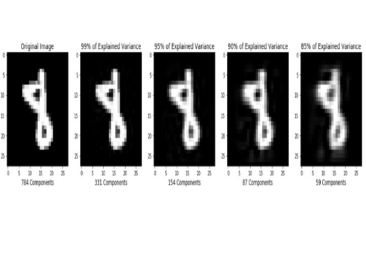
• As expected, the contribution to the total variance decreases dramatically starting from the fifth component, so it's possible to reduce the original dimensionality without an unacceptable loss of information, which could drive an algorithm to learn wrong classes. In the preceding graph, there are the same handwritten digits rebuilt using the first 36 components with whitening and normalization between 0 and 1. • To obtain the original images, we need to inversetransform all new vectors and project them into the original space: >>> X_rebuilt = pca. inverse_transform(X_pca)

The result is shown in the following figure:

Sparse PCA • Finds the set of sparse components that can optimally reconstruct the data. The amount of sparseness is controllable by the coefficient of the L 1 penalty, given by the parameter alpha. • If you think about the handwritten digits or other images that must be classified, their initial dimensionality can be quite high (a 10 x 10 image has 100 features). • However, applying a standard PCA selects only the average most important features, assuming that every sample can be rebuilt using the same components.

On the other hand, we can always use a limited number of components, but without the limitation given by a dense projection matrix. This can be achieved by using sparse matrices (or vectors), where the number of non-zero elements is quite low. In this way, each element can be rebuilt using its specific components Here the non-null components have been put into the first block (they don't have the same order as the previous expression), while all the other zero terms have been separated. In terms of linear algebra, the vectorial space now has the original dimensions.
 >>>")
from sklearn. decomposition import Sparse. PCA >>> spca = Sparse. PCA(n_components=60, alpha=0. 1) >>> X_spca = spca. fit_transform(digits. data / 255) • >>> spca. components_. shape (60 L, 64 L) • The following snippet shows a sparse PCA with 60 components. In this context, they're usually called atoms and the amount of sparsity can be controlled via L 1 -norm regularization (higher alpha parameter values lead to more sparse results).

Kernel PCA • the class Kernel. PCA, which performs a PCA with nonlinearly separable data sets. >>>from sklearn. datasets import make_circles >>> Xb, Yb = make_circles(n_samples=500, factor=0. 1, noise=0. 05) However, looking at the samples and using polar coordinates (therefore, a space where it's possible to project all the points), it's easy to separate the two sets, only considering the radius:

• Considering the structure of the dataset, it's possible to investigate the behavior of a PCA with a radial basis function kernel. • As the default value for gamma is 1. 0/number of features (for now, consider this parameter as inversely proportional to the variance of a Gaussian), we need to increase it to capture the external circle. A value of 1. 0 is enough: >>> from sklearn. decomposition import Kernel. PCA >>> kpca = Kernel. PCA(n_components=2, kernel='rbf', fit_inverse_transform=True, gamma=1. 0) >>> X_kpca = kpca. fit_transform(Xb) The instance variable X_transformed_fit_ will contain the projection of our dataset into the new space. Plotting it, we get:

This example shows that Kernel PCA is able to find a projection of the data that

Atom extraction and dictionary learning • Dictionary learning is a technique which allows rebuilding a sample starting from a sparse dictionary of atoms (similar to principal components). • Is an input dataset and the target is to find both a dictionary D and a set of weights for each sample: • After the training process, an input vector can be computed as: • The optimization problem (which involves both D and alpha vectors) can be expressed as the minimization of the following loss function:

Here the parameter c controls the level of sparsity (which is proportional to the strength of L 1 normalization). This problem can be solved by alternating the least square variable until a stable point is reached. >>>from sklearn. decomposition import Dictionary. Learning >>> dl = Dictionary. Learning(n_components=36, fit_algorithm='lars', transform_algorithm='lasso_lars') >>> X_dict = dl. fit_transform(digits. data) • A plot of each atom (component) is shown in the following figure:

Reference • https: //www. packtpub. com/big-data-andbusiness-intelligence/machine-learningalgorithms
- Slides: 93