Machine Learning BE Computer 2015 PAT A Y

Machine Learning (BE Computer 2015 PAT) A. Y. 2018 -19 SEM-II Prepared by Mr. Dhomse G. P. 1

Unit-1 Introduction to ML Syllabus • classic and adaptive machines 1 hr • Only learning matters 1 hr • Beyond machine learning - deep learning and bio-inspired adaptive systems 1 hr • Machine learning and big data 1 hr • Important Elements in Machine Learning • Data formats ½ hr • Learnability ½ hr • Statistical learning approaches 1 hr • Elements of information theory 1 hr 2

Classic and Adaptive machines The image above roughly explains how Machine Learning works. 3

• Let us say we have a dataset that contains pictures of different kinds of fruits and we want Machine Learning to segregate the photos based on the kind of fruits. • First we provide the dataset to the system i. e we provide the input data. • The system goes through the entire dataset or analyses it to find patterns based on size, shapes, colors, etc. • Now that it has figured out the patterns, the systems takes decisions and starts separating the photos based on the patterns. • Once the work is done, the system learns from the feedback it gets. If it gets any of the fruit type wrong, it will make sure it does not happen in the future. • 4

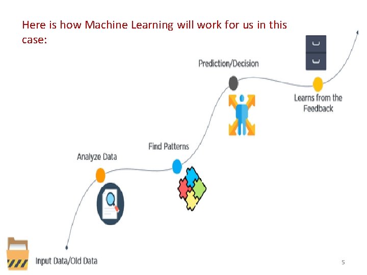
Here is how Machine Learning will work for us in this case: 5

APPLICATIONS OF MACHINE LEARNING • Google Search • Stock Predictions • Robotics-‘Sophia’ introduced which could actually behave like humans. • Social Media Services- Face Recognition , Add as friend in facebook or people you may know • Email Spam and Malware Filtering- C 4. 5 Decision Tree Induction • Over 325, 000 malwares are detected everyday and each piece of code is 90– 98% similar to its previous versions. 6

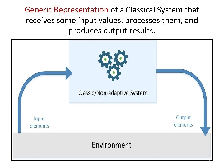
Generic Representation of a Classical System that receives some input values, processes them, and produces output results: • 7

• Machine learning algorithms are described as learning a target function (f) that best maps input variables (X) to an output variable (Y). Y = f(X) • This is a general learning task where we would like to make predictions in the future (Y) given new examples of input variables (X). • It is harder than you think. There is also error (e) that is independent of the input data (X). Y = f(X) + e • This error might be error such as not having enough attributes to sufficiently characterize the best mapping from X to Y. This error is called irreducible error because no matter how good we get at estimating the target function (f), we cannot reduce 8 this error.

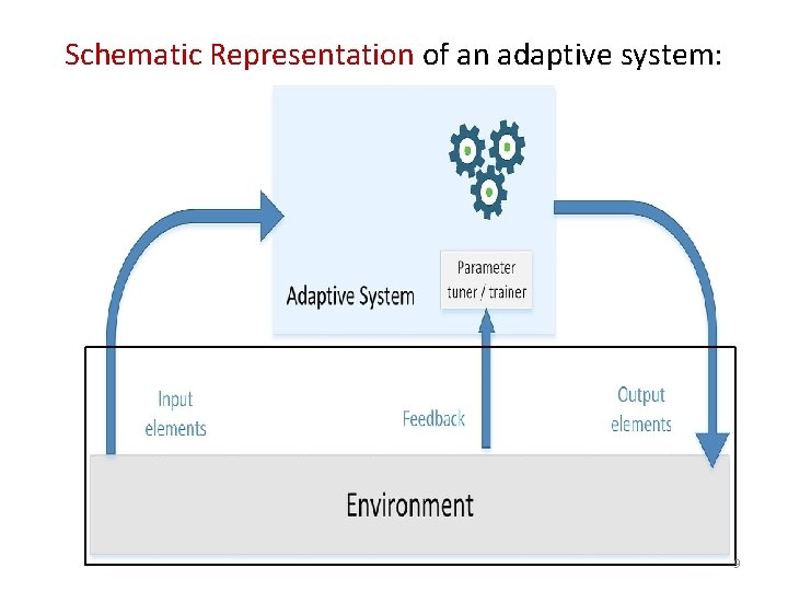
Schematic Representation of an adaptive system: 9

Adaptive Learning- Spam filtering, Natural Language Processing, visual tracking with a webcam or a smartphone, and predictive analysis are only a few applications that revolutionized human-machine interaction and increased our expectations. • Such a system isn't based on static or permanent structures (model parameters and architectures) but rather on a continuous ability to adapt its behavior to external signals (datasets or real-time inputs) and, like a human being, to predict the future using uncertain and fragmentary pieces of information. 10

Machine Learning Matters • Machine learning is to study, engineer, and improve mathematical models which can be trained (once or continuously) with context-related data (provided by a generic environment), to infer the future and to make decisions without complete knowledge of all influencing elements (external factors). • In other words, an agent (which is a software entity that receives information from an environment, picks the best action to reach a specific goal, and observes the results of it) adopts a statistical learning approach, trying to determine the right probability distributions and use them to compute the action (value or decision) that is most likely to be successful (with the least error). 11

Machine learning is a sort of modern magic. • Prediction- Even in the most complex scenarios, such as image classification with convolutional neural networks, every piece of information (geometry, color, peculiar features, contrast, and so on) is already present in the data and the model has to be flexible enough to extract and learn it permanently. 12

Supervised Learning • Supervised learning is where you have input variables (x) and an output variable (Y) and you use an algorithm to learn the mapping function from the input to the output. Y = f(X) • The goal is to approximate the mapping function so well that when you have new input data (x) that you can predict the output variables (Y) for that data. 13

• It is called supervised learning because the process of an algorithm learning from the training dataset can be thought of as a teacher supervising the learning process. • We know the correct answers, the algorithm iteratively makes predictions on the training data and is corrected by the teacher. • Learning stops when the algorithm achieves an acceptable level of performance. 14

• Supervised learning problems can be further grouped into regression and classification problems. • Classification: A classification problem is when the output variable is a category, such as “red” or “blue” or “disease” and “no disease”. • Regression: A regression problem is when the output variable is a real value, such as “dollars” or “weight”. • Some common types of problems built on top of classification and regression include recommendation and time series prediction respectively. • Some popular examples of supervised machine learning algorithms are: • Linear regression for regression problems. • Random forest for classification and regression problems. • Support vector machines for classification problems. 15

Classification example • Sometimes, instead of predicting the actual category, it's better to determine its probability distribution. • For example, an algorithm can be trained to recognize a handwritten alphabetical letter, so its output is categorical (in English, there'll be 26 allowed symbols). • On the other hand, even for human beings, such a process can lead to more than one probable outcome when the visual representation of a letter isn't clear enough to belong to a single category. • That means that the actual output is better described by a discrete probability distribution (for example, with 26 continuous values normalized so that they always sum up to 1). 16

Problem with Supervised learning • overfitting, which causes an overlearning due to an excessive capacity. predict correctly only the samples used for training, while the error for the remaining ones is always very high • ability to 17

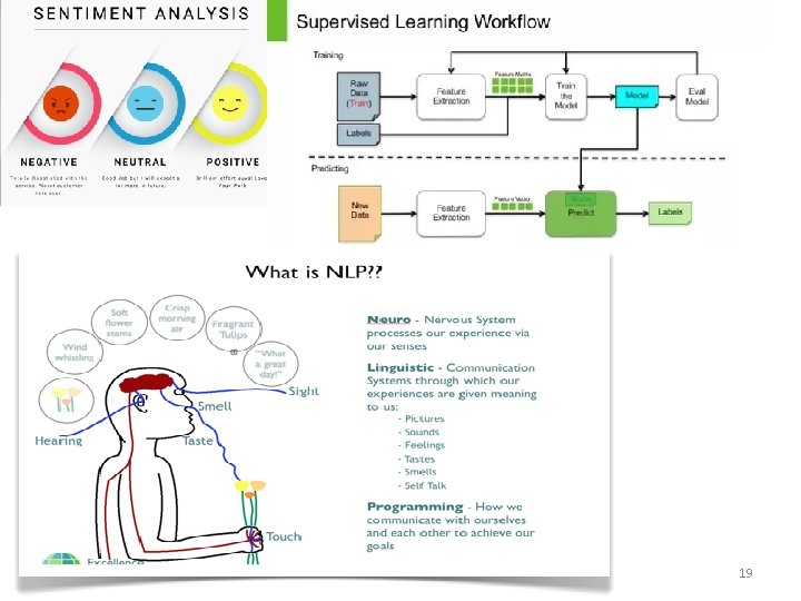
Common Supervised Learning Applications include: • Predictive analysis based on regression or categorical classification Spam detection • Pattern detection • Natural Language Processing • Sentiment analysis • Automatic image classification • Automatic sequence processing (for example, music or speech) 18

19

Unsupervised Machine Learning • Unsupervised learning is where you only have input data (X) and no corresponding output variables. • The goal for unsupervised learning is to model the underlying structure or distribution in the data in order to learn more about the data. • These are called unsupervised learning because unlike supervised learning above there is no correct answers and there is no teacher. Algorithms are left to their own devises to discover and present the interesting structure in the data. 20

• Unsupervised learning problems can be further grouped into clustering and association problems. • Clustering: A clustering problem is where you want to discover the inherent groupings in the data, such as grouping customers by purchasing behavior. • Association: An association rule learning problem is where you want to discover rules that describe large portions of your data, such as people that buy X also tend to buy Y. • Some popular examples of unsupervised learning algorithms are: • k-means for clustering problems. • Apriori algorithm for association rule learning problems. 21

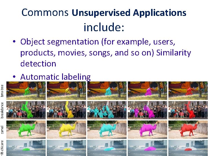
Commons Unsupervised Applications include: • Object segmentation (for example, users, products, movies, songs, and so on) Similarity detection • Automatic labeling 22

Semi-Supervised Machine Learning • Problems where you have a large amount of input data (X) and only some of the data is labeled (Y) are called semi-supervised learning problems. • These problems sit in between both supervised and unsupervised learning. • A good example is a photo archive where only some of the images are labeled, (e. g. dog, cat, person) and the majority are unlabeled. • Many real world machine learning problems fall into this area. This is because it can be expensive or timeconsuming to label data as it may require access to domain experts. Whereas unlabeled data is cheap and 23 easy to collect and store.

Summary • Supervised: All data is labeled and the algorithms learn to predict the output from the input data. • Unsupervised: All data is unlabeled and the algorithms learn to inherent structure from the input data. • Semi-supervised: Some data is labeled but most of it is unlabeled and a mixture of supervised and unsupervised techniques can be used. 24

Reinforcement learning • Reinforcement learning is also based on feedback provided by the environment. However, in this case, the information is more qualitative and doesn't help the agent in determining a precise measure of its error. • this feedback is usually called reward (sometimes, a negative one is defined as a penalty) and it's useful to understand whether a certain action performed in a state is positive or not. 25

an action can also be imperfect, but in terms of a global policy it has to offer the highest total reward. • Reinforcement Learning is a framework for learning where an agent interacts with an environment and receives a reward for each interaction. The goal is to learn to accumulate as much reward as possible over time. • The real advantage these systems have over conventional supervised learning is illustrated by this example I like a lot: • Supervised Learning: Let us say that you know how to play chess. We record you playing games against a lot of people. Now we train a system in the supervised fashion to learn from your examples and call it Kid. Player. Let us say that we train another system on Vishwanathan Anand’s games and call this Pro. Player. Obviously the “policy” learned by Kid. Player will be an inferior player to the policy learned by Pro. Player because of the different capabilities of the teacher. • Reinforcement Learning: In this setting, you make an agent play Chess against someone (usually against another copy of itself) and give it a 26 reward for every time it wins a game.

• to learn the best policy for playing Atari video games and to teach an agent how to associate the right action with an input representing the state (usually a screenshot or a memory dump). • In the following figure, there's a schematic representation of a deep neural network trained to play a famous Atari game. • As input, there are one or more subsequent screenshots (this can often be enough to capture the temporal dynamics as well). • They are processed using different layers (discussed briefly later) to produce an output that represents the policy for a specific state transition. • After applying this policy, the game produces a feedback (as a reward-penalty), and this result is used to refine the output until it becomes stable (so the states are correctly recognized and the suggested action is always the best one) and the total 27 reward overcomes a predefined threshold.

Atari Video Game 28

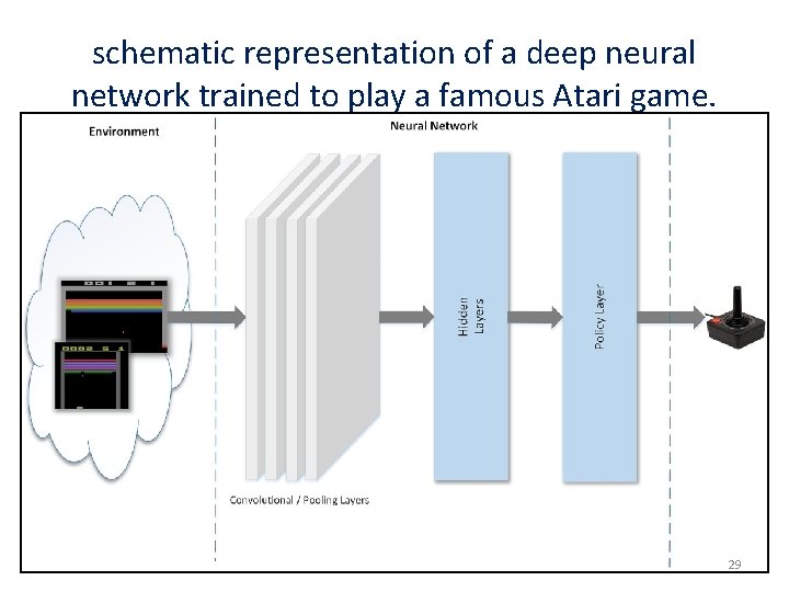
schematic representation of a deep neural network trained to play a famous Atari game. 29

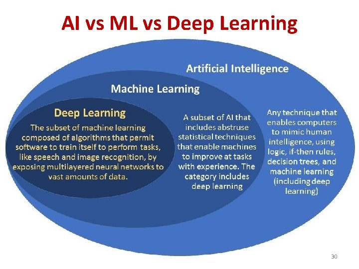
AI vs ML vs Deep Learning 30

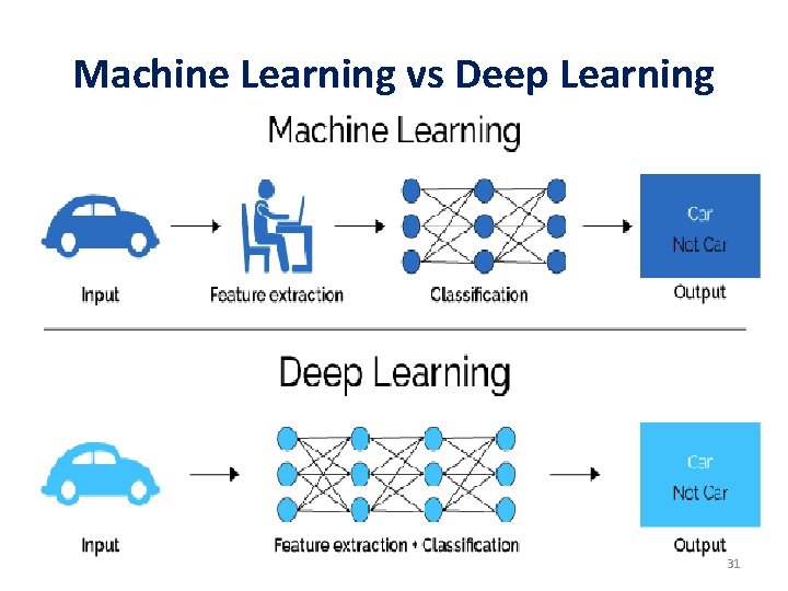
Machine Learning vs Deep Learning 31

Deep Learning • Machine learning concerned with algorithms inspired by the structure and function of the brain called artificial neural networks. • A deep neural network (DNN) is an artificial neural Network (ANN) with multiple hidden layers between the input and output layers. • DNNs are typically feedforward networks in which data flows from the input layer to the output layer without looping back. • where as feedforward with Backpropagation ( is a common method for training a neural network in back direction with change of weights according to error) forms a better DNN. • Recurrent neural networks (RNNs), in which data can flow in any direction, are used for applications for language purposes. • Convolutional neural networks (CNNs) are used in computer vision. CNNs have been applied to acoustic modeling for 32 automatic speech recognition

Beyond Machine Learning - Deep Learning and bio-inspired adaptive systems • many researchers started training bigger and bigger models, built with several different layers (that's why this approach is called deep learning), to solve new challenging problems. • The availability of cheap and fast computers allowed them to get results in acceptable timeframes and to use very large datasets (made up of images, texts, and animations). 33

• The idea behind these techniques is to create algorithms that work like a brain • neurosciences and cognitive psychology. • In particular, there's a growing interest in pattern recognition and associative memories whose structure and functioning are similar to what happens in the neocortex. Such an approach also allows simpler algorithms called model- free • It is based on generic learning techniques and repeating experiences. • testing different architectures and optimization algorithms is quite simpler 34

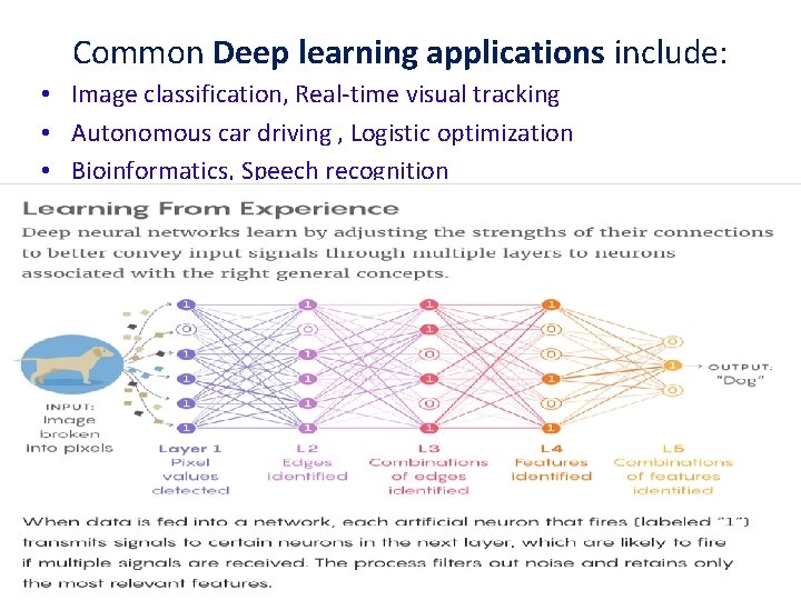
Common Deep learning applications include: • Image classification, Real-time visual tracking • Autonomous car driving , Logistic optimization • Bioinformatics, Speech recognition 35

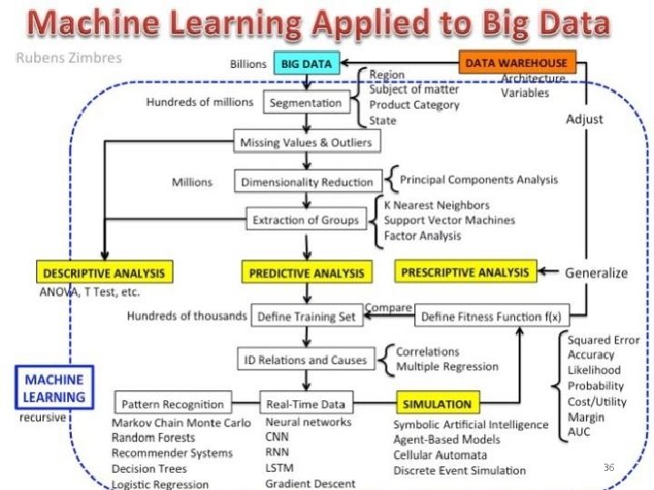
36

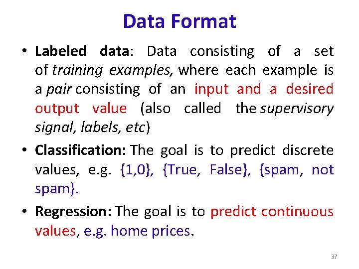
Data Format • Labeled data: Data consisting of a set of training examples, where each example is a pair consisting of an input and a desired output value (also called the supervisory signal, labels, etc) • Classification: The goal is to predict discrete values, e. g. {1, 0}, {True, False}, {spam, not spam}. • Regression: The goal is to predict continuous values, e. g. home prices. 37

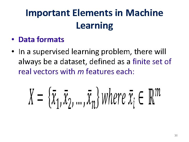
Important Elements in Machine Learning • Data formats • In a supervised learning problem, there will always be a dataset, defined as a finite set of real vectors with m features each: 38

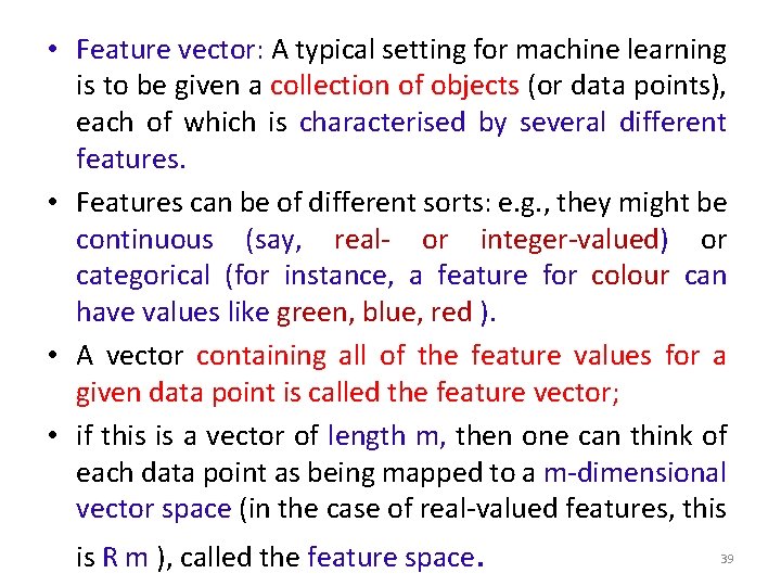
• Feature vector: A typical setting for machine learning is to be given a collection of objects (or data points), each of which is characterised by several different features. • Features can be of different sorts: e. g. , they might be continuous (say, real- or integer-valued) or categorical (for instance, a feature for colour can have values like green, blue, red ). • A vector containing all of the feature values for a given data point is called the feature vector; • if this is a vector of length m, then one can think of each data point as being mapped to a m-dimensional vector space (in the case of real-valued features, this is R m ), called the feature space. 39

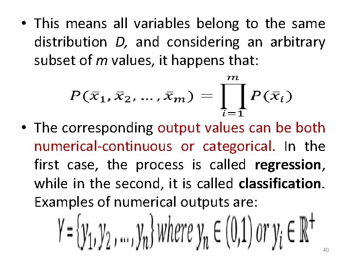
• This means all variables belong to the same distribution D, and considering an arbitrary subset of m values, it happens that: • The corresponding output values can be both numerical-continuous or categorical. In the first case, the process is called regression, while in the second, it is called classification. Examples of numerical outputs are: 40

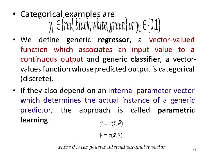
• Categorical examples are • We define generic regressor, a vector-valued function which associates an input value to a continuous output and generic classifier, a vectorvalues function whose predicted output is categorical (discrete). • If they also depend on an internal parameter vector which determines the actual instance of a generic predictor, the approach is called parametric learning: 41

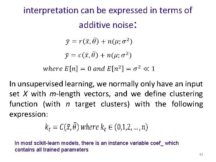
interpretation can be expressed in terms of additive noise: In unsupervised learning, we normally only have an input set X with m-length vectors, and we define clustering function (with n target clusters) with the following expression: In most scikit-learn models, there is an instance variable coef_ which contains all trained parameters 42

Multiclass strategies • When the number of output classes is greater than one, there are two main possibilities to manage a classification problem: • One-vs-all- If there are n output classes, n classifiers will be trained in parallel considering there is always a separation between an actual class and the remaining ones. • This approach is relatively lightweight (at most, n-1 checks are needed to find the right class, so it has an O(n) complexity) and, for this reason, it's normally the default choice and there's no need for further actions. 43

• One-vs-one • The alternative to one-vs-all is training a model for each pair of classes. • The complexity is no longer linear (it's O(n 2) indeed) and the right class is determined by a majority vote. • In general, this choice is more expensive and should be adopted only when a full dataset comparison is not preferable. 44

Learnability • 45

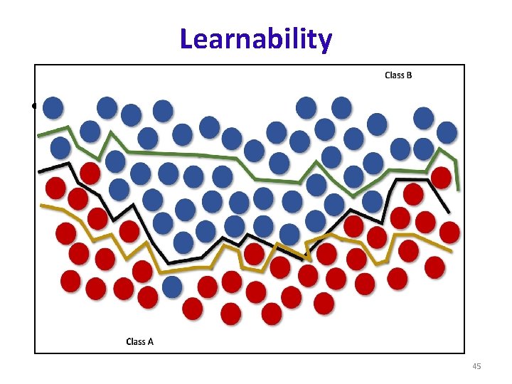
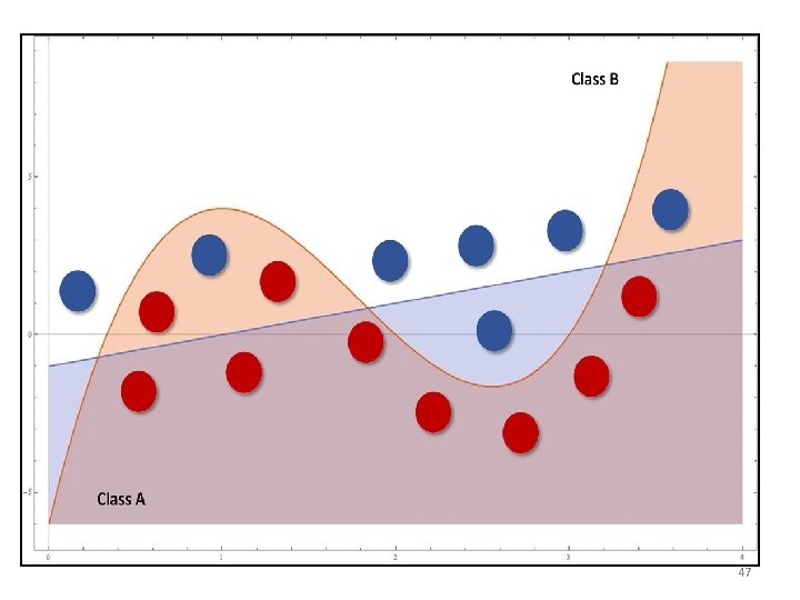
• there's an example of a dataset whose points must be classified as red (Class A) or blue (Class B). • Three hypotheses are shown: the first one (the middle line starting from left) misclassifies one sample, • while the lower and upper ones misclassify 13 and 23 samples respectively: • the first hypothesis is optimal and should be selected; however, it's important to understand an essential concept which can determine a potential overfitting 46

47

• The blue classifier is linear while the red one is cubic. At a glance, non-linear strategy seems to perform better, because it can capture more expressivity, thanks to its concavities. • However, if new samples are added following the trend defined by the last four ones (from the right), they'll be completely misclassified. • In fact, while a linear function is globally better but cannot capture the initial oscillation between 0 and 4, a cubic approach can fit this data almost perfectly but, at the same time, loses its ability to keep a global linear trend. 48

Underfitting and overfitting • Underfitting: It means that the model isn't able to capture the dynamics shown by the same training set (probably because its capacity is too limited). • Overfitting: the model has an excessive capacity and it's not more able to generalize considering the original dynamics provided by the training set. It can associate almost perfectly all the known samples to the corresponding output values, but when an unknown input is presented, the corresponding prediction error can be very high. 49

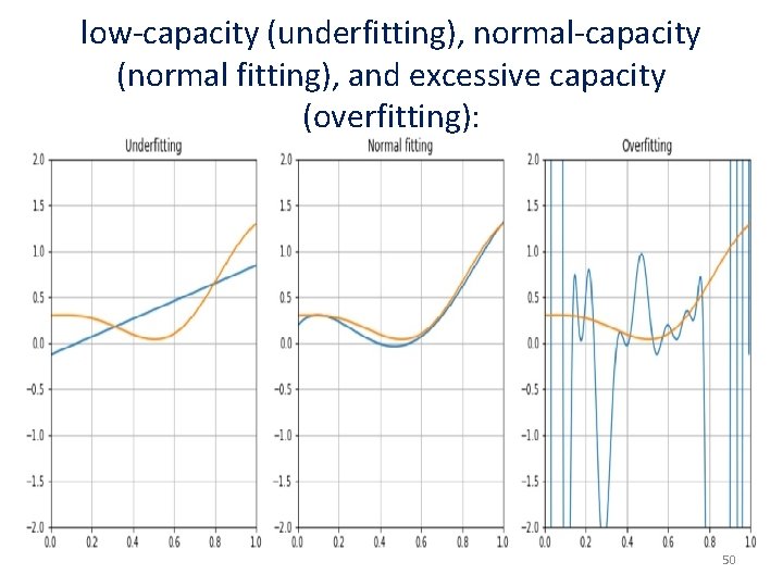
low-capacity (underfitting), normal-capacity (normal fitting), and excessive capacity (overfitting): 50

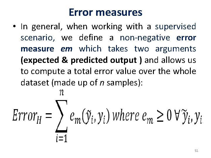
Error measures • In general, when working with a supervised scenario, we define a non-negative error measure em which takes two arguments (expected & predicted output ) and allows us to compute a total error value over the whole dataset (made up of n samples): 51

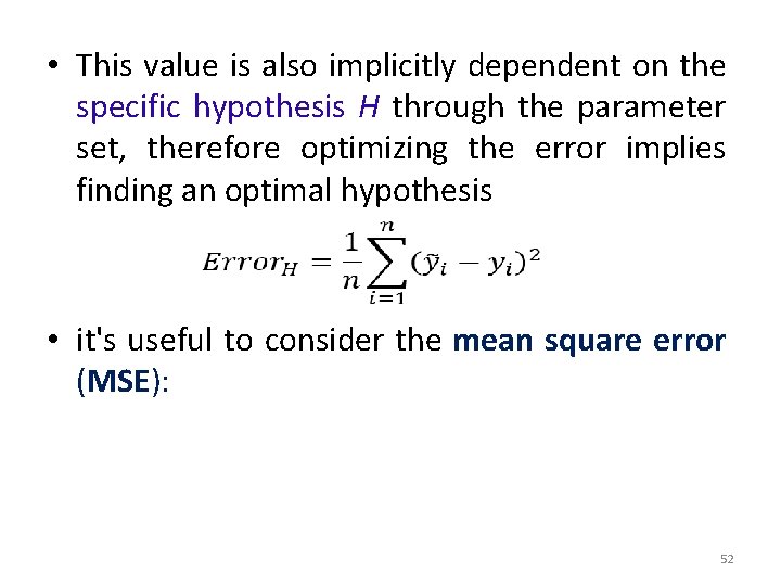
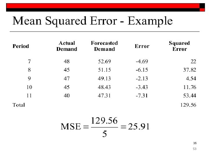
• This value is also implicitly dependent on the specific hypothesis H through the parameter set, therefore optimizing the error implies finding an optimal hypothesis • it's useful to consider the mean square error (MSE): 52

53

• This measure is also called loss function because its value must be minimized through an optimization problem. • When it's easy to determine an element which must be maximized, the corresponding loss function will be its reciprocal. • Another useful loss function is called zero-one -loss and it's particularly efficient for binary classifications (also for one-vs-rest multiclass strategy): 54

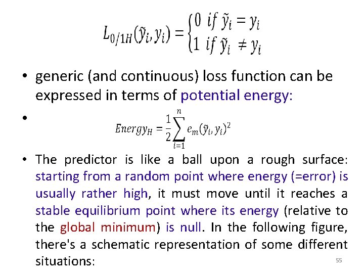
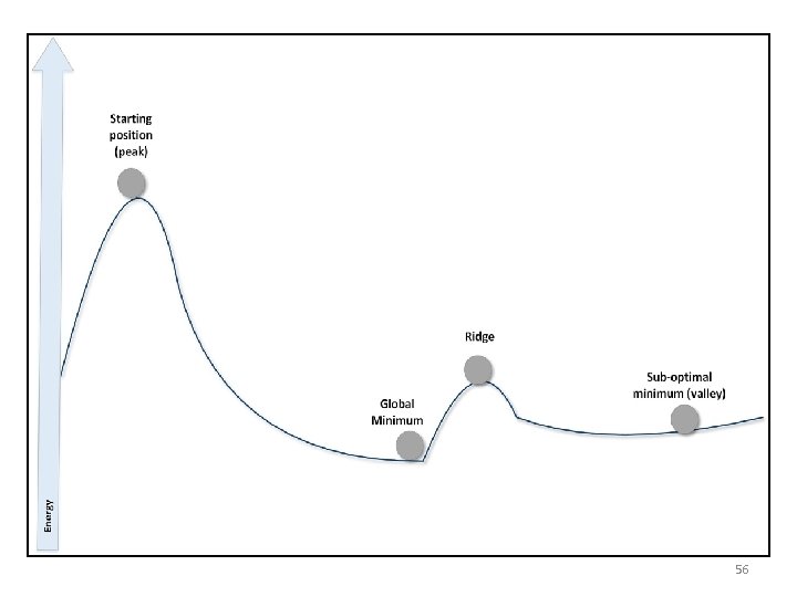
• generic (and continuous) loss function can be expressed in terms of potential energy: • • The predictor is like a ball upon a rough surface: starting from a random point where energy (=error) is usually rather high, it must move until it reaches a stable equilibrium point where its energy (relative to the global minimum) is null. In the following figure, there's a schematic representation of some different 55 situations:

56

• the starting point is stable without any external perturbation, so to start the process, it's needed to provide initial kinetic energy. • However, if such an energy is strong enough, then after descending over the slope the ball cannot stop in the global minimum. • The residual kinetic energy can be enough to overcome the ridge and reach the right valley. If there are not other energy sources, the ball gets trapped in the plain valley and cannot move anymore. • avoid local minima. However, every situation must always be carefully analyzed to understand what level of residual energy (or error) is acceptable, or whether it's better to adopt a different strategy 57

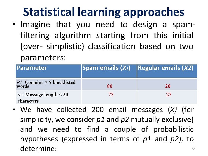
Statistical learning approaches • Imagine that you need to design a spamfiltering algorithm starting from this initial (over- simplistic) classification based on two parameters: Parameter P 1 Contains > 5 blacklisted words p 2 - Message length < 20 characters Spam emails (X 1) Regular emails (X 2) 80 20 75 25 • We have collected 200 email messages (X) (for simplicity, we consider p 1 and p 2 mutually exclusive) and we need to find a couple of probabilistic hypotheses (expressed in terms of p 1 and p 2), to 58 determine:

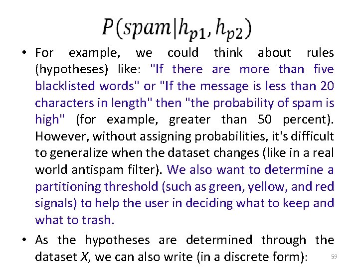
• For example, we could think about rules (hypotheses) like: "If there are more than five blacklisted words" or "If the message is less than 20 characters in length" then "the probability of spam is high" (for example, greater than 50 percent). However, without assigning probabilities, it's difficult to generalize when the dataset changes (like in a real world antispam filter). We also want to determine a partitioning threshold (such as green, yellow, and red signals) to help the user in deciding what to keep and what to trash. • As the hypotheses are determined through the 59 dataset X, we can also write (in a discrete form):

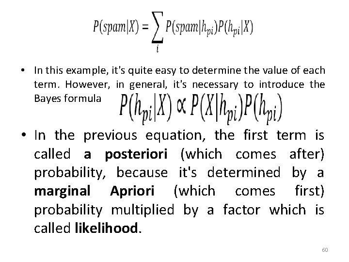
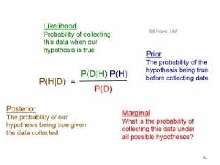
• In this example, it's quite easy to determine the value of each term. However, in general, it's necessary to introduce the Bayes formula • In the previous equation, the first term is called a posteriori (which comes after) probability, because it's determined by a marginal Apriori (which comes first) probability multiplied by a factor which is called likelihood. 60

61

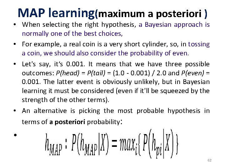
MAP learning(maximum a posteriori ) • When selecting the right hypothesis, a Bayesian approach is normally one of the best choices, • For example, a real coin is a very short cylinder, so, in tossing a coin, we should also consider the probability of even. • Let's say, it‘s 0. 001. It means that we have three possible outcomes: P(head) = P(tail) = (1. 0 - 0. 001) / 2. 0 and P(even) = 0. 001. The latter event is obviously unlikely, but in Bayesian learning it must be considered (even if it'll be squeezed by the strength of the other terms). • An alternative is picking the most probable hypothesis in terms of a posteriori probability: • 62

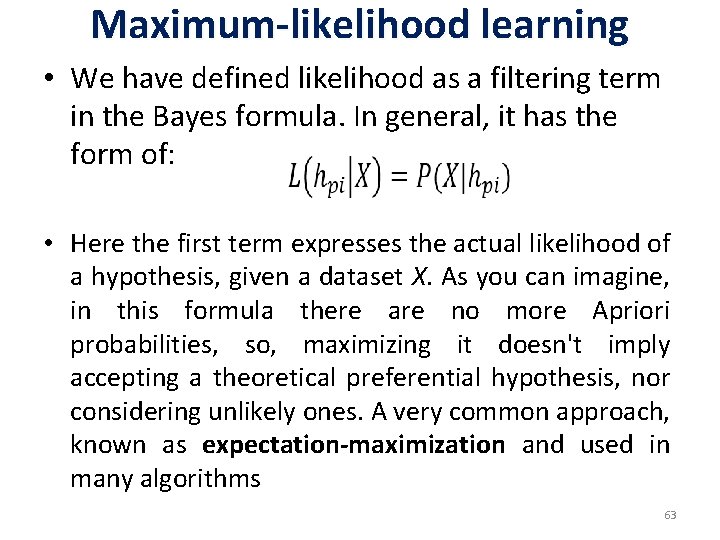
Maximum-likelihood learning • We have defined likelihood as a filtering term in the Bayes formula. In general, it has the form of: • Here the first term expresses the actual likelihood of a hypothesis, given a dataset X. As you can imagine, in this formula there are no more Apriori probabilities, so, maximizing it doesn't imply accepting a theoretical preferential hypothesis, nor considering unlikely ones. A very common approach, known as expectation-maximization and used in many algorithms 63

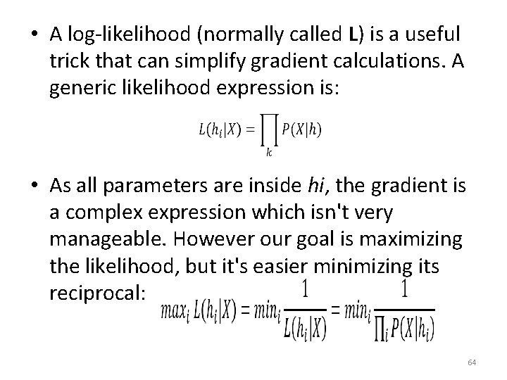
• A log-likelihood (normally called L) is a useful trick that can simplify gradient calculations. A generic likelihood expression is: • As all parameters are inside hi, the gradient is a complex expression which isn't very manageable. However our goal is maximizing the likelihood, but it's easier minimizing its reciprocal: 64

Elements of information theory • A machine learning problem can also be analyzed in terms of information transfer or exchange. Our dataset is composed of n features, which are considered independent (for simplicity, even if it's often a realistic assumption) drawn from n different statistical distributions. • Therefore, there are n probability density functions pi(x) which must be approximated through other n qi(x) functions. • In any machine learning task, it's very important to understand how two corresponding distributions diverge and what is the amount of information we lose when approximating the original dataset. 65

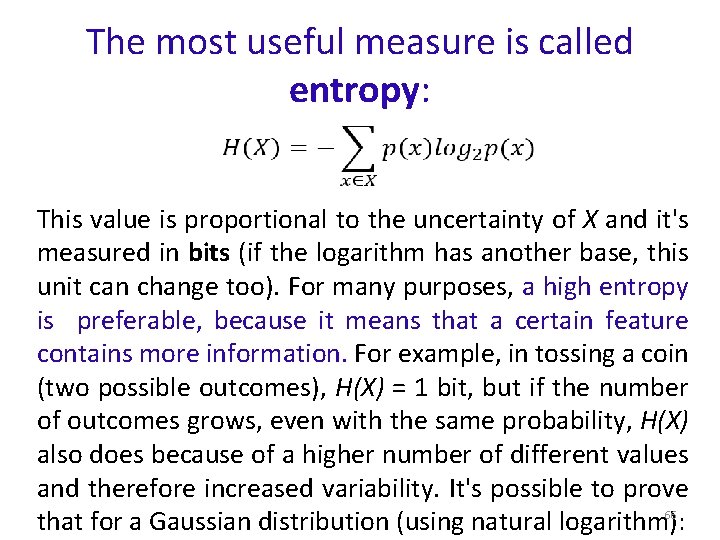
The most useful measure is called entropy: This value is proportional to the uncertainty of X and it's measured in bits (if the logarithm has another base, this unit can change too). For many purposes, a high entropy is preferable, because it means that a certain feature contains more information. For example, in tossing a coin (two possible outcomes), H(X) = 1 bit, but if the number of outcomes grows, even with the same probability, H(X) also does because of a higher number of different values and therefore increased variability. It's possible to prove 66 that for a Gaussian distribution (using natural logarithm):

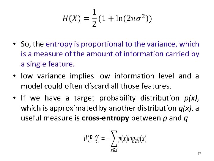
• So, the entropy is proportional to the variance, which is a measure of the amount of information carried by a single feature. • low variance implies low information level and a model could often discard all those features. • If we have a target probability distribution p(x), which is approximated by another distribution q(x), a useful measure is cross-entropy between p and q 67

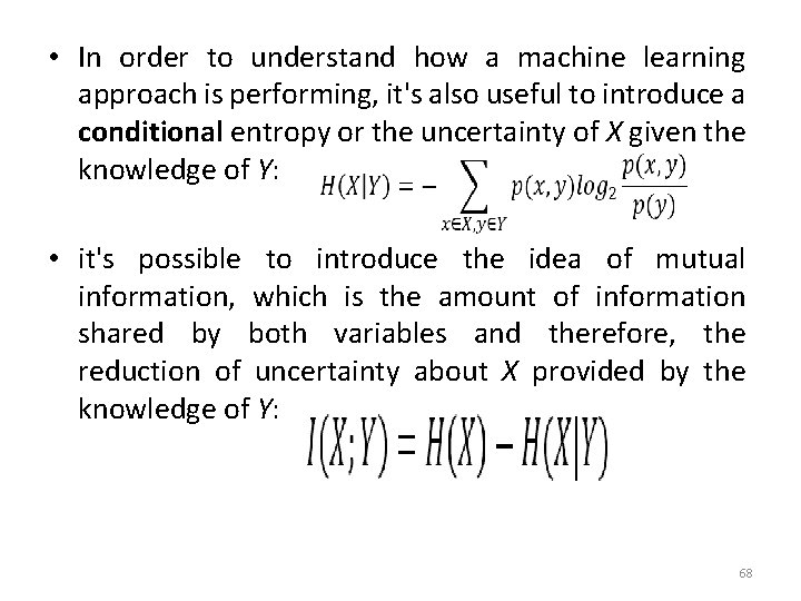
• In order to understand how a machine learning approach is performing, it's also useful to introduce a conditional entropy or the uncertainty of X given the knowledge of Y: • it's possible to introduce the idea of mutual information, which is the amount of information shared by both variables and therefore, the reduction of uncertainty about X provided by the knowledge of Y: 68

• Intuitively, when X and Y are independent, they don't share any information. However, in machine learning tasks, there's a very tight dependence between an original feature and its prediction, so we want to maximize the information shared by both distributions. • If the conditional entropy is small enough (so Y is able to describe X quite well), the mutual information gets close to the marginal entropy H(X), which measures the amount of information we want to learn. 69

References • • • Russel S. , Norvig P. , Artificial Intelligence: A Modern Approach, Pearson Valiant L. , A Theory of the Learnable, Communications of the ACM, Vol. 27, No. 11 (Nov. 1984) Hastie T. , Tibshirani R. , Friedman J. , The Elements of Statistical Learning: Data Mining, Inference and, Prediction, Springer Aleksandrov A. D. , Kolmogorov A. N, Lavrent'ev M. A. , Mathematics: Its contents, Methods, and Meaning, Courier Corporation https: //www. packtpub. com/big-data-and-business-intelligence/machine-learningalgorithms 70