Machine learning and model ensembling allow for the

Machine learning and model ensembling allow for the development of a generic and performant NIRS calibration pipeline Cornet D. (Cirad), Desfontaines L. (INRA), Ehounou E. (CNRA), Cormier F. (Cirad), Marie-Magdeleine C. (INRA), Arnau G. (Cirad), Kouakou A. (CNRA), Davrieux F. (Cirad), Beurier G. (Cirad) RTBfoods 1 st Annual Meeting, March 21 -27 th, Abuja, Nigeria WP 3 Side-meeting on HTP Methods 20 March 2019 © D. Cornet (CIRAD)

Content • Justification of the methodology choice • Ensembling techniques at hand • Analysis pipeline under development • Perspectives

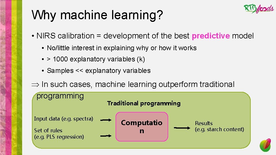
Why machine learning? • NIRS calibration = development of the best predictive model • No/little interest in explaining why or how it works • > 1000 explanatory variables (k) • Samples << explanatory variables Þ In such cases, machine learning outperform traditional programming Traditional programming Input data (e. g. spectra) Set of rules (e. g. PLS regression) Computatio n Results (e. g. starch content)

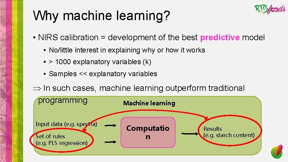
Why machine learning? • NIRS calibration = development of the best predictive model • No/little interest in explaining why or how it works • > 1000 explanatory variables (k) • Samples << explanatory variables Þ In such cases, machine learning outperform traditional programming Machine learning Input data (e. g. spectra) Set of rules (e. g. PLS regression) Computatio n Results (e. g. starch content)

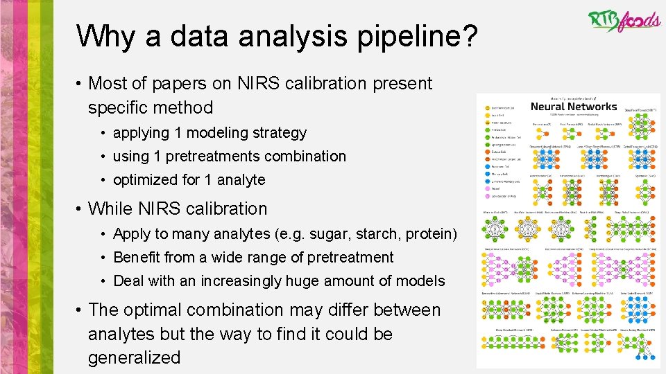
Why a data analysis pipeline? • Most of papers on NIRS calibration present specific method • applying 1 modeling strategy • using 1 pretreatments combination • optimized for 1 analyte • While NIRS calibration • Apply to many analytes (e. g. sugar, starch, protein) • Benefit from a wide range of pretreatment • Deal with an increasingly huge amount of models • The optimal combination may differ between analytes but the way to find it could be generalized

Why ensembling models? • Diversity of combinations of Pretreatments/Models/Analytes • A single best model • may not benefit from all the information leading to its choice • may adapt too much to the training dataset noise (overfitting) • Vast majority of winning team in science competition contest (kaggle) do not use best single model but a combination of many models • This base models combination into a meta algorithm is called model ensembling. • First used in 1992 by Wolpert but its advantage was only mathematically demonstrated in 2007 (van de Laar et al. )

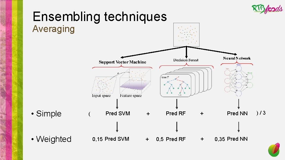
Ensembling techniques Averaging • Simple • Weighted ( Pred SVM + Pred RF + Pred NN 0, 15 Pred SVM + 0, 5 Pred RF + 0, 35 Pred NN )/3

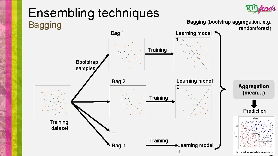
Ensembling techniques Bagging Bag 1 Bagging (bootstrap aggregation, e. g. randomforest) Learning model 1 Training Bootstrap samples Learning model 2 Bag 2 Training Aggregation (mean…) Prediction Training dataset …. Bag n Training Learning model n https: //towardsdatascience. c

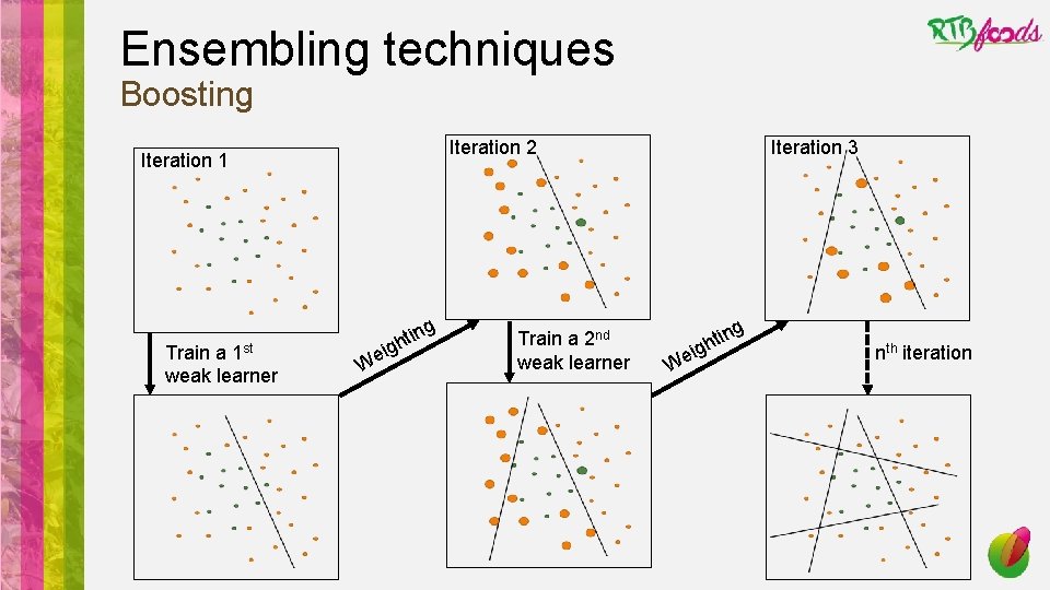
Ensembling techniques Boosting Iteration 2 Iteration 1 Train a 1 st weak learner ig e W ng i t h Train a 2 nd weak learner Iteration 3 g ig e W n hti nth iteration

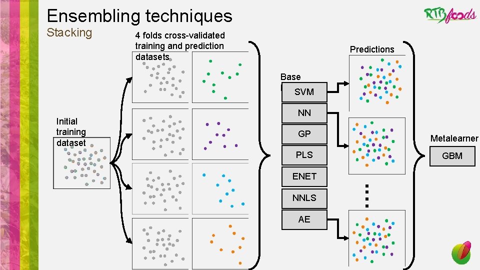
Ensembling techniques Stacking 4 folds cross-validated training and prediction datasets Predictions Base learners SVM Initial training dataset NN GP Metalearner PLS GBM ENET AE . … NNLS

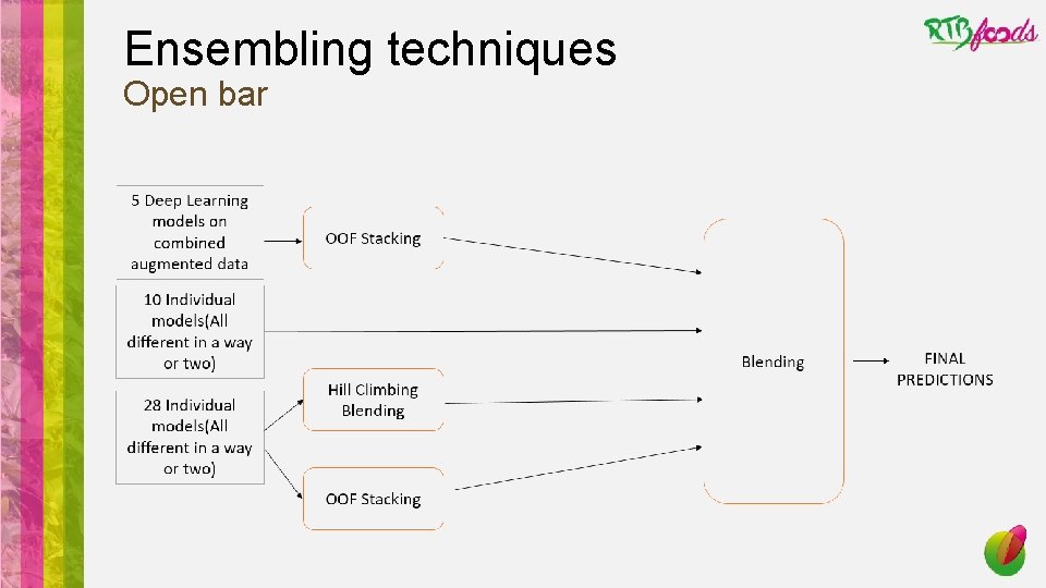
Ensembling techniques Open bar

Ensembling techniques How to enhance performance of the meta algorithme? • Base models have to be • Diverse: the higher the diversity of base models the lower the bias in the ensemble model (e. g. avoiding tree based models). • Performant: Models with uniform and high performances (>< old fashion weak learner) • Trade-off between these two traits => hard to avoid highly correlated models while choosing highly performant ones.

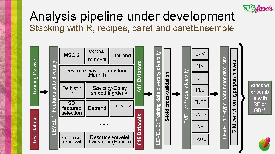
Analysis pipeline under development Derivativ e … Continuum removal Descrete wavelet transform (Haar 5) PLS ENET NNLS AE Lasso Grid search on hyperparameters Detrend GP LEVEL 4 : Hyperparameter diversity SD features selection Savitsky-Golay smoothing/deriv. NN LEVEL 3: Model diversity Derivativ e SVM 5 -fold cross-validation Descrete wavelet transform (Haar 1) LEVEL 2: Training data diversity removal Detrend 615 Datasets Continuu m 615 Datasets MSC 2 LEVEL 1: Features sets diversity Test Dataset Training Dataset Stacking with R, recipes, caret and caret. Ensemble Stacked ensemb le with RF or GBM

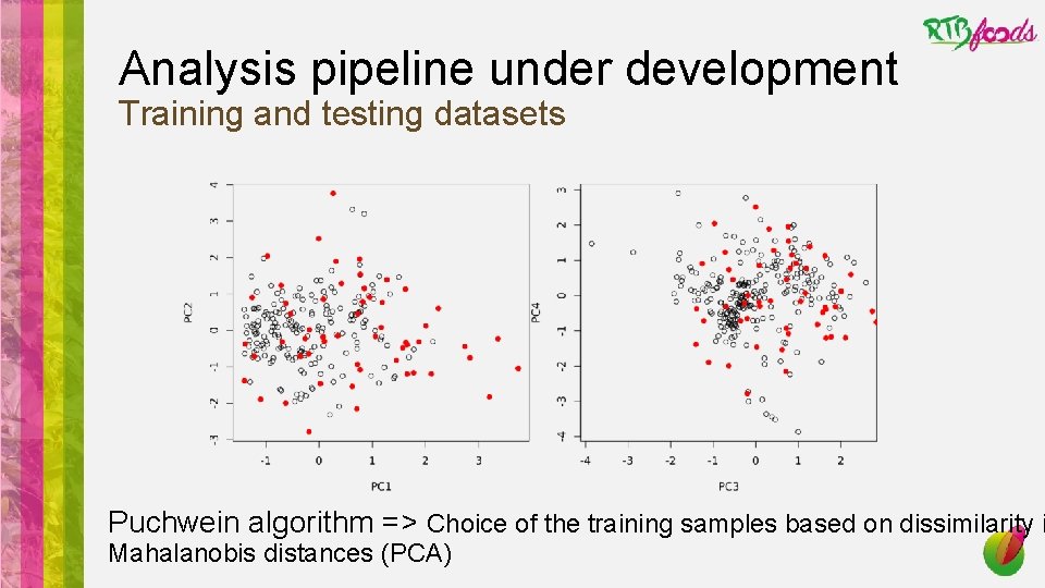
Analysis pipeline under development Training and testing datasets Puchwein algorithm => Choice of the training samples based on dissimilarity i Mahalanobis distances (PCA)

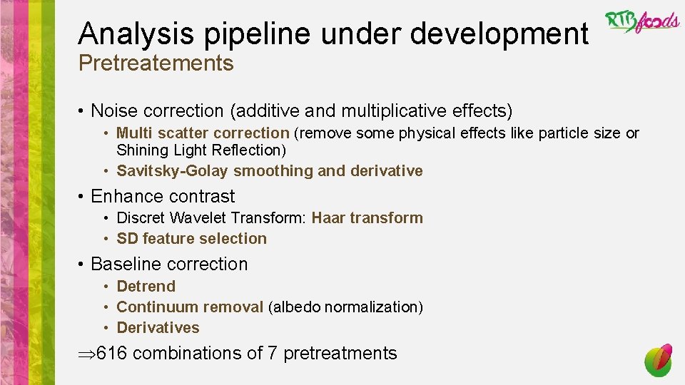
Analysis pipeline under development Pretreatements • Noise correction (additive and multiplicative effects) • Multi scatter correction (remove some physical effects like particle size or Shining Light Reflection) • Savitsky-Golay smoothing and derivative • Enhance contrast • Discret Wavelet Transform: Haar transform • SD feature selection • Baseline correction • Detrend • Continuum removal (albedo normalization) • Derivatives Þ 616 combinations of 7 pretreatments

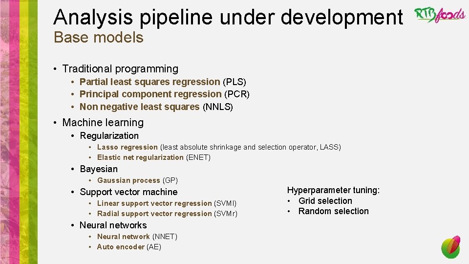
Analysis pipeline under development Base models • Traditional programming • Partial least squares regression (PLS) • Principal component regression (PCR) • Non negative least squares (NNLS) • Machine learning • Regularization • Lasso regression (least absolute shrinkage and selection operator, LASS) • Elastic net regularization (ENET) • Bayesian • Gaussian process (GP) • Support vector machine • Linear support vector regression (SVMl) • Radial support vector regression (SVMr) • Neural networks • Neural network (NNET) • Auto encoder (AE) Hyperparameter tuning: • Grid selection • Random selection

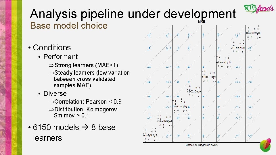
Analysis pipeline under development Base model choice • Conditions • Performant ÞStrong learners (MAE<1) ÞSteady learners (low variation between cross validated samples MAE) • Diverse ÞCorrelation: Pearson < 0. 9 ÞDistribution: Kolmogorov. Smirnov > 0. 1 • 6150 models 8 base learners

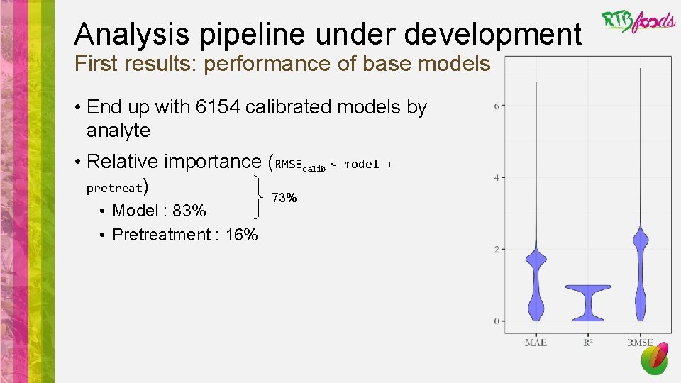
Analysis pipeline under development First results: performance of base models • End up with 6154 calibrated models by analyte • Relative importance (RMSEcalib ~ pretreat) • Model : 83% • Pretreatment : 16% 73% model +

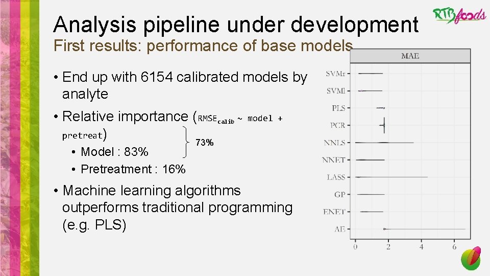
Analysis pipeline under development First results: performance of base models • End up with 6154 calibrated models by analyte • Relative importance (RMSEcalib ~ pretreat) • Model : 83% • Pretreatment : 16% model + 73% • Machine learning algorithms outperforms traditional programming (e. g. PLS)

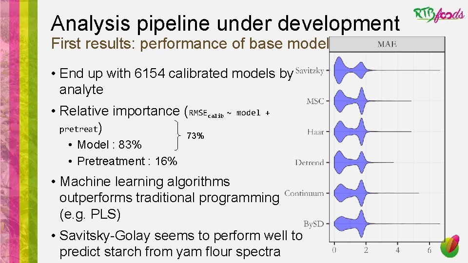
Analysis pipeline under development First results: performance of base models • End up with 6154 calibrated models by analyte • Relative importance (RMSEcalib ~ pretreat) • Model : 83% • Pretreatment : 16% model + 73% • Machine learning algorithms outperforms traditional programming (e. g. PLS) • Savitsky-Golay seems to perform well to predict starch from yam flour spectra

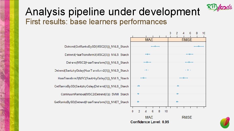
Analysis pipeline under development First results: base learners performances

Perspectives • Finalize the coding of the analysis pipeline • Play with post analysis results: look at relative performance of pretreatments/models/analytes • Test the genericity of our pipeline on different crops, products, dataset size • Test the added value of working on a vector of analytes rather than sequentially treat every single analyte (better handling of outliers and noise, synergic effect while linked analytes…) • Adding mid-infrared spectroscopy to NIRS spectra • Improve the speed of the pipeline using other libraries (e. g. keras, h 2 o) or languages (e. g. python) • Test next generation deep learning algorithms which are able to mimic pretreatments (e. g. RNN, CNN, LSTM, attention based NN)

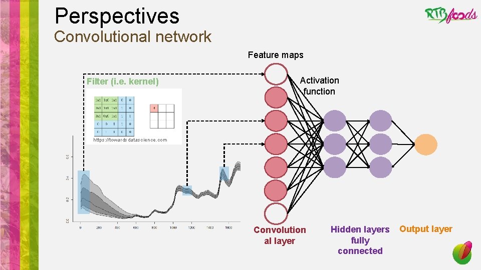
Perspectives Convolutional network Feature maps Filter (i. e. kernel) Activation function https: //towardsdatascience. com Convolution al layer Hidden layers fully connected Output layer

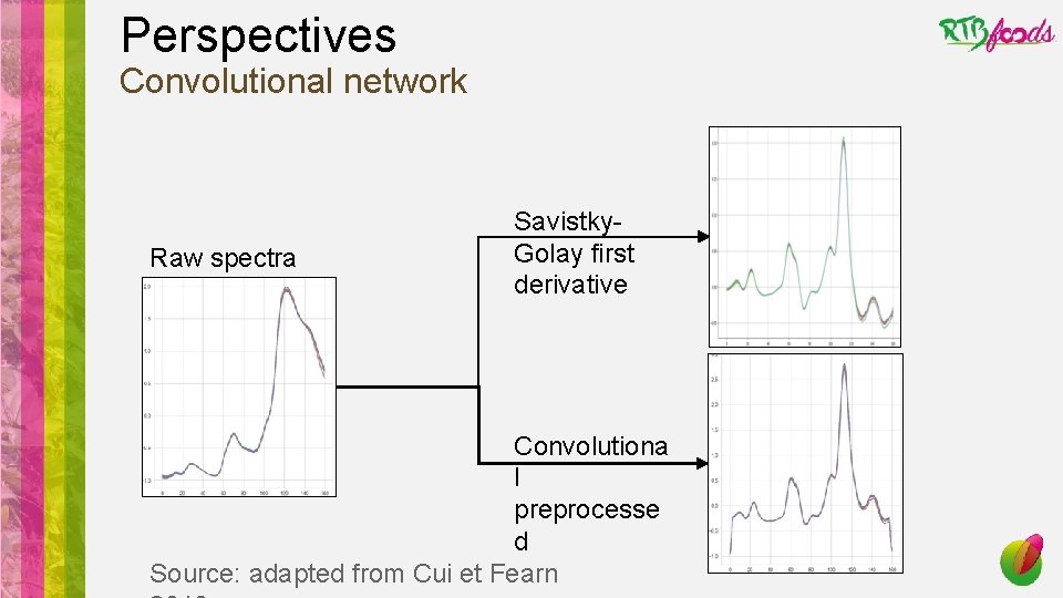
Perspectives Convolutional network Raw spectra Savistky. Golay first derivative Convolutiona l preprocesse d Source: adapted from Cui et Fearn

Thank you