Machine Design II Unit VI Sliding Contact Bearings

Machine Design II Unit VI Sliding Contact Bearings Prof. R. S. Hingole Professor and Head Mechanical Engg. Deptt. DYPCOE Akurdi. Pune e

BEARING It supports the rotating element Types of Bearings 1. Depending upon the direction of load to be supported i) Radial ii) Thrust 2. Depending upon the nature of contact i) Sliding contact a) Journal b) Thrust i) Rolling contact a) Cylindrical b) Taper c) Needle

SLIDING CONTACT BEARINGS: 1) To support a rotating member viz. , a shaft. 2) Transmit the load from a rotating member to a stationary member known as frame or housing 3) Permit relative motion of two members

1. 2 SLIDING CONTACT BEARINGS - ADVANTAGES AND DISADVANTAGES These bearings have certain advantages over the rolling contact bearings. They are: 1. The design of the bearing and housing is simple. 2. They occupy less radial space and are more compact. 3. They cost less. 4. The design of shaft is simple. 5. They operate more silently. 6. They have good shock load capacity. 7. They are ideally suited for medium and high speed operation. The disadvantages are: 1. The frictional power loss is more. 2. They required good attention to lubrication. 3. They are normally designed to carry radial load or axial load only.

1. 3 SLIDING CONTACT BEARINGS CLASSIFICATION Sliding contact bearings are classified in three ways. 1. Based on type of load carried 2. Based on type of lubrication 3. Based on lubrication mechanism

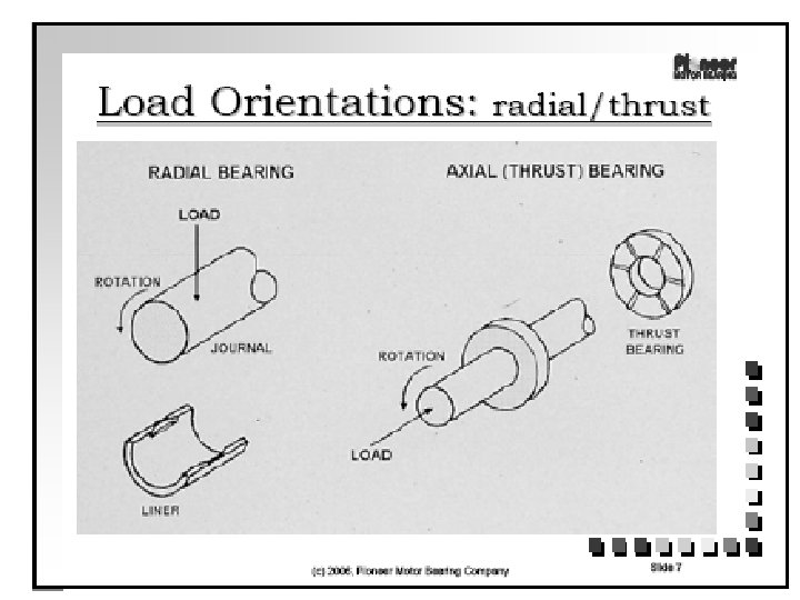
1. 3. 1 Bearing classification based on type of load carried a. Radial bearings b. Thrust bearings or axial bearings c. Radial – thrust bearings 1. 3. 1(a) Radial bearings These bearings carry only radial loads. Fig. 1. 1 Radial Bearing

i) Radial Bearing • Load acts perpendicular to direction of motion

Physical Characteristics of Radial Bearings These bearings have one row of balls; also known as single row. 1. It has two rings namely an outer and an inner ring, which is placed inside the outer ring. 2. The inner ring is placed in such a way that it touches the outer ring at one point with the rings oriented in the same direction. 3. A crescent-shaped open area is formed between the rings. 4. With relation to the outer ring, the inner ring is snapped back to its original position. 5. The retainer is fitted in place and the balls are evenly distributed in the raceway. 6. The balls settle to the deepest point of the raceway when a radial load is applied to the bearing.

Advantages of Radial Ball Bearings Corrosion resistant Lightweight Non-metallic and non-magnetic with glass balls Maintenance free Low friction Lubrication free Bearing and application integration Design flexibility Low inertia- freer turning Applications Of Radial Ball Bearings Manufacturing aircraft components such as engines, wing flaps, rod-ends, wing mounts and hatches. Motors, hand tools, fans, etc. Helicopters, trains and automobiles, functioning as joints.

1. 3. 1(b) Thrust or axial bearings These bearings carry only axial loads Fig. 1. 2(a) Single collar thrust Bearing Fig. 1. 2(b) Multiple collar thrust Bearing

1. 3. 1(c) Radial thrust bearings These bearings carry both radial and thrust loads.

i) Thrust Bearing • • Load acts along axis of rotation of shaft Thrust bearing is a particular type of rotary bearing

1. 3. 2. Bearing classification based on type of lubrication The type of lubrication means the extent to which the contacting surfaces are separated in a shaft bearing combination. This classification includes (a) Thick film lubrication (b) Thin film lubrication (c) Boundary lubrication

(a) Thick film lubrication (a) the surfaces are separated by thick film of lubricant and there will not be any metal-to-metal contact. (b) The film thickness is anywhere from 8 to 20 μm. Typical values of coefficient of friction are 0. 002 to 0. 010. (c) Hydrodynamic lubrication is coming under this category. Wear is the minimum.

b) Thin film lubrication – The surfaces are separated by thin film of lubricant, at some high spots Metal-to-metal contact does exist , Because of this intermittent contacts, it also known as mixed film lubrication. Surface wear is mild. The coefficient of friction commonly ranges from 0. 004 to 0. 10.

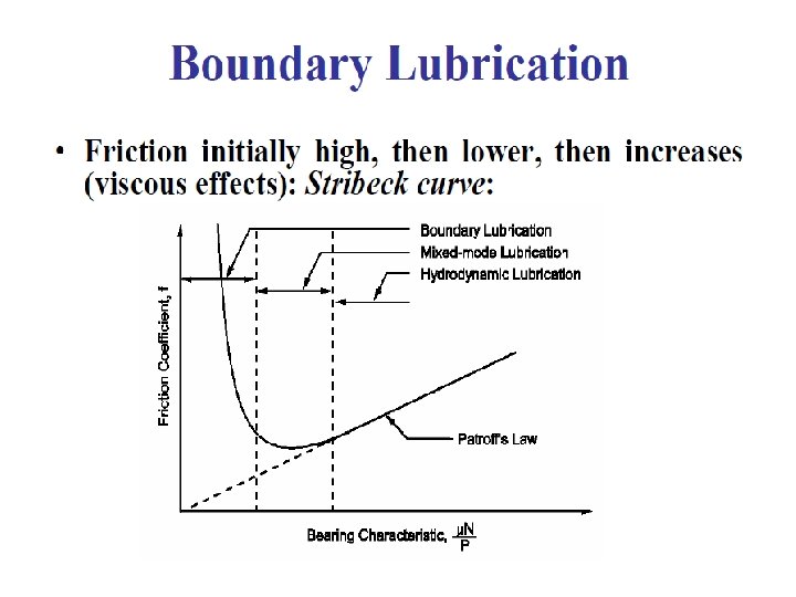
(c). Boundary lubrication – Here the surface contact is continuous and extensive as Shown in Fig. The lubricant is continuously smeared over the surfaces and provides a continuously renewed adsorbed surface film which reduces the friction and wear. The typical coefficient of friction is 0. 05 to 0. 20.

1. 3. 3 Bearing classification based on lubrication mechanism a. Hydrodynamic lubricated bearings b. Hydrostatic lubricated bearings c. Elastohydrodynamic lubricated bearings d. Boundary lubricated bearings e. Solid film lubricated bearings

1. 3. 3(a) Hydrodynamic lubricated bearings The load-carrying surfaces are separated by a stable thick film of lubricant that prevents the metal-to-metal contact. The film pressure generated by the moving surfaces that force the lubricant through a wedge shaped zone. At sufficiently high speed the pressure developed around the journal sustains the load. This is illustrated in Fig. 1. 6.

1. 5 HYDRODYNAMIC LUBRICATION In 1883 Beauchamp Tower discovered that when a bearing is supplied with adequate oil, a pressure is developed in the clearance space when the journal rotates about an axis that is eccentric with the bearing axis. He exhibited that the load can be sustained by this fluid pressure without any contact between the two members. The load carrying ability of a hydrodynamic bearing arises simply because a viscous fluid resists being pushed around. Under proper conditions, this resistance to motion will develop a pressure distribution in the film that can support useful load. Two mechanisms responsible for this are wedge film and squeeze film action.

1. 5. 1 Stages in hydrodynamic lubrication Consider a steady load F, a fixed bearing and a rotating journal. Stage 1 –: At rest, the bearing clearance space is filled with oil, but the load F has squeezed out the oil film at the bottom. Metal-to-contact exists. The vertical axis of bearing and journal are co-axial. Load and reaction are in line fig. 1. 10.

Stage 2: When the journal starts rotating slowly in clockwise direction, because of friction, the journal starts to climb the wall of the bearing surface as in Fig. 1. 11. Boundary lubrication exists now. The wear normally takes place during this period. However, the journal rotation draws the oil between the surfaces and they separate.

Stage 3: As the speed increases, more oil is drawn in and enough pressure is built up in the contact zone to float” the journal Fig. 1. 12. Further increase in speed, additional pressure of the converging oil flow to the right of the minimum film thickness position (ho) moves the shaft slightly to the left of center.

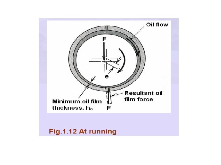
As a result full separation of journal and bearing surfaces occurs. In stable operating condition, the pressure distribution on the journal is shown in Fig. 1. 13. This is known as – Hydrodynamic lubrication or full film/thick film lubrication. At this equilibrium condition, the pressure force on journal balances the external load F.

1. 5. 2 HYDRODYNAMIC LUBRICATION - ANIMATION 1. 5. 3 The friction characteristics of hydrodynamic lubrication of journal bearings Average pressure on project surface of the journal: p = F / (l*d) -----------(1. 1) Where F – Radial load l – Length of the journal d – Journal diameter ld - Bearing projected area

2. Depending upon the nature of contact i) Sliding contact a) Journal b) Thrust a) Journal

i) Rolling contact a) Cylindrical b) Taper c) Needle a) Fig. Cylindrical bearing

b) Fig. Taper bearing

c) Fig. Needle Roller bearing

2. 1 PETROFF’S EQUATION FOR BEARING FRICTION In 1883, Petroff published his work on bearing friction based on simplified assumptions. a. No eccentricity between bearings and journal and hence there is no “Wedging action” as in Fig. 2. 1. b. Oil film is unable to support load. c. No lubricant flow in the axial direction. Fig. 2. 1 Unloaded Journal bearing

With reference to Fig. 2. 1, an expression for viscous friction drag torque is derived by considering the entire cylindrical oil film as the “liquid block” acted upon by force F. From Newton’s law of Viscosity: F = μ * AU/h ------2. 1 Fig. 2. 2 Laminar flow of fluid in clearance space

Where F = friction torque/shaft radius = 2 T f / d A= π d l U = π d n (Where n is in rps d is in m) h = c (Where c = radial clearance = 0. 5(D-d)) r = d /2 Substituting and solving for friction torque: Tf = f 4π2 μnlr 3 /c (2. 2) If a small radial load W is applied to the shaft, Then the frictional drag force f w and the friction Torque will be: Tf = f w = 0. 5 f (d l p) d (2. 3)

Equating eon. (2. 2) and (2. 3) and simplifying, we get Where r = 0. 5 d and u is Pa. This is known as Petroff’s equation for bearing friction. It gives reasonable estimate of co-efficient of friction of lightly loaded bearings. The first quantity in the bracket stands for bearing modulus and second one stands for clearance ratio. Both are dimensionless parameters of the bearing. Clearance ratio normally ranges from 500 to 1000 in bearings.

2. 3 HYDRODYNAMIC LUBRICATION THEORY Beauchamp Tower’s exposition of hydrodynamic behavior of journal bearings in 1880 s and his observations drew the attention of Osborne Reynolds to carryout theoretical analysis. This has resulted in a fundamental equation for hydrodynamic lubrication. This has provided a strong foundation and basis for the design of hydro-dynamic lubricated bearings.

In his theoretical analysis, Reynolds made the following assumptions: a) The fluid is Newtonian. b) The fluid is incompressible. c) The viscosity is constant throughout the film. d) The pressure does not vary in the axial direction. e) The bearing and journal extend infinitely in the z direction. i. e. , no lubricant flow in the z direction. f) The film pressure is constant in the y direction. Thus the pressure depends on the x coordinate only. g) The velocity of particle of lubricant in the film depends only on the coordinates x and y. h) The effect of inertial and gravitational force is neglected. i) The fluid experience laminar flow.

2. 3. 1 Reynolds’ Equation As shown in Fig. 2. 4, the Forces acting on a fluid element of height dy, width dx, velocity u, and top to bottom velocity gradient du is considered.

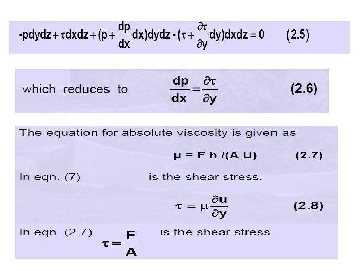
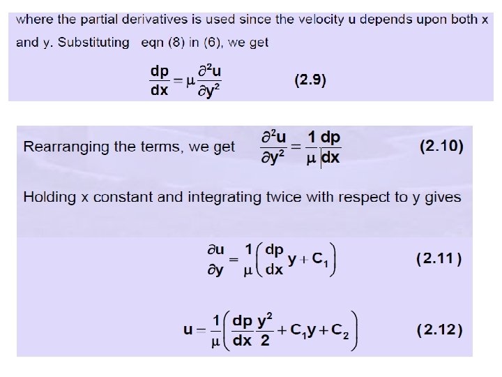
Fig. 2. 5 Pressure and viscous forces acting on an element of lubricant. Only X components are shown

The assumption of no slip between the lubricants and the boundary surfaces gives boundary conditions enabling C 1 and C 2 to be evaluated: u=0 at y=0, u=U at y=h

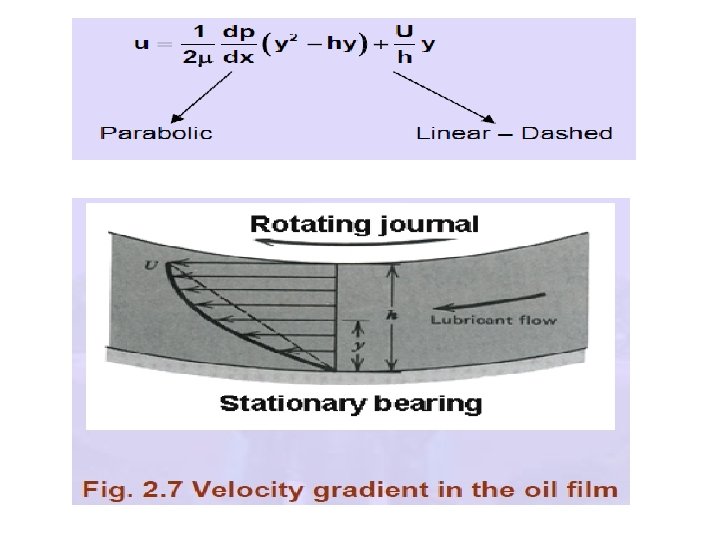
Fig. 2. 6 Velocity distribution in the oil film Velocity Distribution of the Lubricant Film shown in Fig. 2. 6 consists of two terms on the right hand side.

At the section when pressure is a maximum and the velocity gradient is linear. Let the volume of lubricant per-unit time flowing across the section containing the element in Fig. 2. 6. For unit width in the Z direction, Let the volume of lubricant per-unit time flowing across the section containing the element in Fig. 2. 6 be Qf. For unit width in the Z direction,

For an in-compressible liquid, the flow rate must be the same for all cross sections, which means that Differentiating equation (2. 16) with respect to x and equating to zero, This is the classical Reynolds’ equation for one dimensional flow. This is valid for long bearings.

In short bearings, flow in the Z direction or end leakage has to be taken into account. A similar development gives the Reynolds’ Equation for two dimensional flows: Modern bearings are short and (l / d) ratio is in the range 0. 25 to 0. 75. This causes flow in the z direction (the end leakage) to a large extent of the total flow. For short bearings, Ockvirk has neglected the x terms and simplified the Reynolds’ equation as:

Unlike previous equations (2. 19) and (2. 20), equation (2. 21) can be readily integrated and used for design and analysis purpose. The procedure is known as Ocvirk’s short bearing approximation.

2. 4 DESIGN CHARTS FOR HYDRODYNAMIC BEARINGS Solutions to eqn. 2. 19 were developed in first decade of 20 th century and were applicable for long bearings and give reasonably good results for bearings with (l / d) ratios more than 1. 5. Ocvirk’s short bearing approximation on the other hand gives accurate results for bearings with (l /d) ratio up to 0. 25 and often provides reasonable results for bearings with (l / d) ratios between 0. 25 and 0. 75.

Raimondi and Boyd have obtained computerized solutions for Reynolds eqn. (2. 20) and reduced them to chart form which provide accurate solutions for bearings of all proportions. Selected charts are shown in Figs. 2. 8 to 2. 15. All these charts are plots of non-dimensional bearing parameters as functions of the bearing characteristic number, or the Sommerfeld variable S which itself is a dimensionless parameter.

Fig. 2. 8 Chart for minimum film thickness variable and eccentricity ratio. The left shaded zone defines the optimum ho for minimum friction; the right boundary is the optimum ho for maximum load

Fig. 2. 9 Chart for determining the position of the minimum film thickness ho for location refer Fig. 2. 10

Fig. 2. 10 Stable hydrodynamic lubrication

Fig. 2. 11 Chart for coefficient of friction variable.

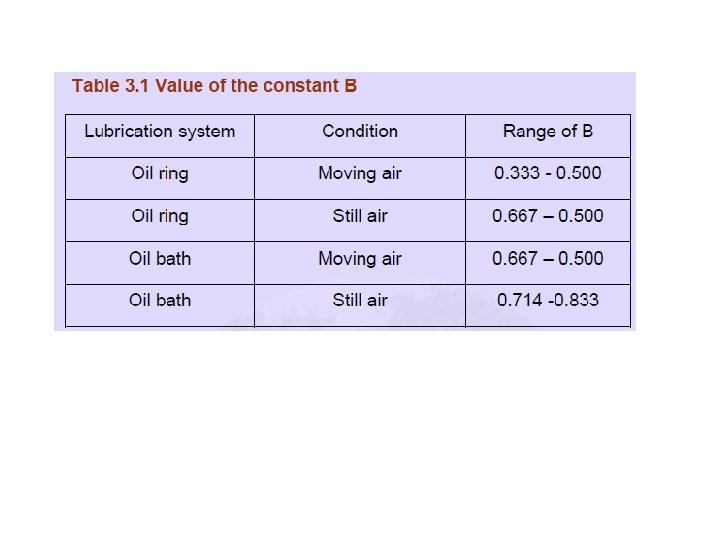
3. 5 HYDRODYNAMIC LUBRICATED JOURNAL BEARING DESIGN The following guidelines aid in design: 3. 5. 1 Unit loading The load per unit journal projected area is denoted by p. In many applications like engine bearings, momentary peak loads result in bearing pressures of the order of ten times the steady state values. The hydrodynamic bearings can take up such peak loads without any problem. The recommended values of steady unit load for various applications are given in Table 3. 1. This helps in selecting suitable diameter for any particular the application.

3. 5. 2 Bearing l / d ratios Ratios - 0. 25 to 0. 75 are now commonly used in modern machinery whereas in older machinery closer to unity was used. Longer bearings have less end leakage and reduced oil flow requirements and high oil temperature. Short bearings are less prone to edge loading from shaft deflection and misalignments, need higher flow rate and run cooler. The shaft size is found from fatigue strength and rigidity considerations. Bearing length is found from permissible unit loads. Table 3. 2 Unit loads for journal bearings

(b) Rapidly fluctuating loads p = Fmax / d l

2. 3. 1 Raimondi and Boyd Equation There is no exact solution for Reynolds equation for a journal bearing having a finite length. However A A Raimondi and John Boyd have solved intergration tech by using digital computer

Radi al clearence c is C = R-r ----------------1 Clearence = radius of bearing – radius of journal The eccentricity ratio (Ɛ) Ɛ = e/c-------2 From fig R = e+r+h 0 ---------------a Where ho = min film thickness (mm) Put eq a in eq 1

Put eq a in eq 1 C = e+r+h 0 -r C = e+ho = Ɛc+h 0 Or C(1 - Ɛ) = ho Ɛ = 1 - (ho/c) -----------------3 (ho/c) = Min film thickness variable The summerfield no. is given by S = (r/c)2 - (µ ns / P) ------------4

S = summerfield no. µ = viscosity of lub (Ns/mm 2) ns = Journal speed (rev/sec) P= Unit bearing pressure (N/mm 2) CV (coe of friction variable ) = (r/c) f f = coe of friction