LYRA the Lymanalpha Radiometer onboard PROBA2 LYRA Tests

LYRA the Lyman-alpha Radiometer onboard PROBA-2 LYRA Tests and Calibration LYRA Meeting Davos 05/06 Oct 2006

Contents I. From Model to Configuration II. BESSY Campaigns a. Flux Linearity b. Stability, Drift c. LEDs, Dark Current d. Spectral Responsivity e. Homogeneity, Flatfield f. Cadence, Response Time III. Summary IV. Additional Topics
, Aluminium,")
I. From Model to Configuration Choice of filters: Zirconium (150 nm, 300 nm), Aluminium, Lyman-alpha (N, XN, VN, and combinations thereof), Herzberg, … Choice of detectors: MSMxx (diamond), PINxx (diamond), AXUVxx (silicon), … - Tested separately to find transmittance and responsivity - Simulated with TIMED-SEE solar spectra to find expected response values and purities cf. http: //lyra. oma. be/radiometric_model. php Example: “high” flux + “Herzberg” filter + “PIN” detector

Selected configurations: filter detector nominal FWHM measured 1 -1 Ly XN 1 -2 Herzberg 1 -3 Aluminium 1 -4 Zr (300 nm) + + MSM 12 PIN 10 MSM 11 AXUV 20 D 121. 5 +/- nm 200 -220 nm 17 -80 nm 1 -20 nm 116 -126 nm 197 -218 nm (1)-2. 4, 17 -35 nm (1)-1. 3, 6 -15 nm 2 -1 Ly XN 2 -2 Herzberg 2 -3 Aluminium 2 -4 Zr (150 nm) + + MSM 21 PIN 11 MSM 15 MSM 19 121. 5 +/- nm 200 -220 nm 17 -80 nm 1 -20 nm 116 -126 nm 199 -219 nm (1)-1. 4, 17 -27 nm (1)-1. 3, 6 -12 nm 3 -1 Ly N+XN 3 -2 Herzberg 3 -3 Aluminium 3 -4 Zr (300 nm) + + AXUV 20 A PIN 12 AXUV 20 B AXUV 20 C 121. 5 +/- nm 200 -220 nm 17 -80 nm 1 -20 nm 116 -126 nm 198 -219 nm (1)-2. 4, 17 -35 nm (1)-1. 3, 6 -15 nm

Consequence: - All channels individual - No simple redundancy - Combined responsivities - New estimates for response and purity (cf. II d. )
 July 2005")
II. BESSY Campaigns - NI beamline (40 – 240 nm, 60 C) July 2005 Doc. RP-ROB-LYR-0132 -NI-July 2005 - GI beamline (1 – 30 nm, 60 C) July 2005 Doc. RP-ROB-LYR-0132 -GI-July 2005 - (Final) NI beamline (40 – 240 nm, 37 C) March 2006 Doc. RP-ROB-LYR-0132 -NI-March 2006 - (Final) GI beamline (1 – 30 nm, 37 C) March 2006 Doc. RP-ROB-LYR-0132 -GI-March 2006

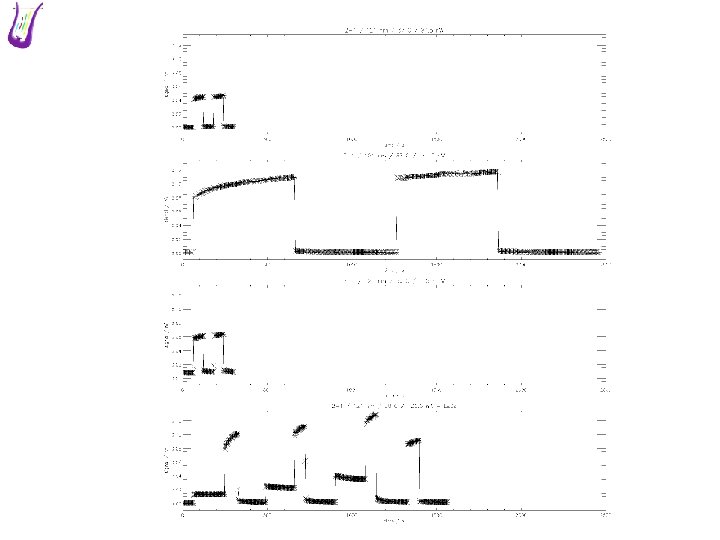
a. Flux Linearity - Using different aperture stops, or - Varying exit slit of monochromator - Relation fitted (2006) with a function I=[c+]a*P^b - Results: almost linear, slightly sub/superlinear, sub/superlinear (qualitatively) - or: b~1, c~0 (quantitatively)
 GI 2005 (20 nm,")
Results in detail: NI 2006 (121. 6 nm, 200 nm) GI 2005 (20 nm, 10 nm) NI 2006 (121. 6 nm, 210 nm, 50 nm) (18 nm, 10 nm) 1 -1 MSM slightly sublin. 1 -2 PIN slightly superlin. 1 -3 MSM 1 -4 AXUV 0. 99572 1. 00656 0. 98565 2 -1 MSM 2 -2 PIN 2 -3 MSM 2 -4 MSM 1. 03661 0. 99483 1. 02234 slightly sublin. slightly superlin. 3 -1 AXUV almost linear 3 -2 PIN almost linear 3 -3 AXUV 3 -4 AXUV superlinear slightly superlin. sublinear almost linear GI 2006 1. 02434 0. 99529 0. 00230 1. 1719, but c>0 1. 00155 0. 97894 1. 04009 0. 99253 1. 00064

b. Stability, Drift - Shutter was opened and closed every 60 s, then every 600 s - Some additional longer tests were executed - BESSY 2005 campaigns (60 C) still to be analyzed in detail - LED values, dark current values and 44 C, 50 C temperature effects: see below Example: Channel 2 -1 (Ly XN + MSM 21) at BESSY NI 2006
 in detail: start drift (“slow” ~min, “almost immediate” ~s) stop (“tail” ~min,")
Results (2006) in detail: start drift (“slow” ~min, “almost immediate” ~s) stop (“tail” ~min, “almost immediate” ~s) 1 -1 MSM 1 -2 PIN 1 -3 MSM 1 -4 AXUV slow almost immediate, slow immediate upward (almost) no upward no tail almost immediate tail, almost immediate 2 -1 MSM 2 -2 PIN 2 -3 MSM 2 -4 MSM slow almost immediate slow upward (almost) no upward tail immediate almost immediate 3 -1 AXUV 3 -1 3 -2 PIN 3 -3 AXUV 3 -4 AXUV (almost) immediate almost immediate (almost) no no almost immediate (almost) immediate almost immediate

c. LEDs, Dark Current 1 -1 MSM 1 -2 PIN 1 -3 MSM 1 -4 AXUV 2 -1 MSM 2 -2 PIN 2 -3 MSM 2 -4 MSM 3 -1 AXUV 3 -2 PIN 3 -3 AXUV 3 -4 AXUV vis. LED uv. LED offset @37 C (0. 005) 0. 004 (0. 100) (0. 024) 0. 014 0. 001 0. 000, -0. 007 -0. 004 (0. 012) (0. 023) 0. 015 -0. 001 ((0. 016 -0. 136)) 0. 000? 0. 006 (1. 059) 0. 000 0. 001 -0. 002 0. 000, -0. 008 -0. 001 0. 002 -0. 003 -0. 001, -0. 011 -0. 014 44 C 50 C 0. 003 0. 010 -0. 002 0. 010 0. 002 0. 009 -0. 005 0. 007 -0. 003 0. 008 -0. 005 All values in n. A (x) = varying around x, ((x-y)) = unstable from y to x, “negative” current values due to conversion
 Relevant spectral")
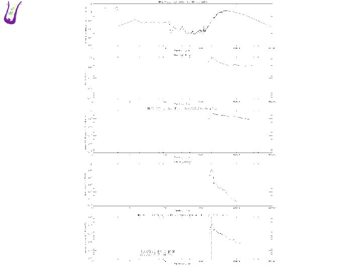
d. Spectral Responsivity - Filters and detectors measured together (“channels” as configurated) Relevant spectral range is tested, with special attention to range borders V changed to A using appropriate gain resistor Corrections for ring current applied Example: “high” solar flux simulated with measurements of channel 1 -1 (Ly XN + MSM 12) at BESSY NI 2006 - How to estimate “correction factors”? Consequences for data levels?
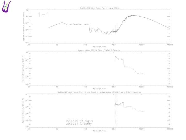

Expected Signal and Purity theorectical: “min” “high” measured: “min” “high” 1 -1 MSM 0. 139 n. A (37%) 1 -2 PIN 12. 75 n. A (86%) 1 -3 MSM 0. 120 n. A (61%) 1 -4 AXUV 0. 530 n. A (99%) 0. 161 n. A (44%) 12. 77 n. A (86%) 5. 264 n. A ( 3%) 15. 37 n. A (88%) 0. 240 n. A (24%) 0. 267 n. A (30%) 12. 57 n. A (83%) 12. 59 n. A (83%) 0. 086 n. A (58%) 4. 945 n. A ( 3%) 0. 699 n. A (100%) 19. 09 n. A (100%) 2 -1 MSM 2 -2 PIN 2 -3 MSM 2 -4 MSM 0. 135 n. A (46%) 13. 82 n. A (83%) 3. 821 n. A ( 6%) 2. 878 n. A (100%) 0. 104 n. A (21%) 0. 114 n. A (26%) 13. 75 n. A (84%) 13. 76 n. A (84%) 0. 074 n. A (59%) 3. 837 n. A ( 3%) 0. 094 n. A (100%) 2. 772 n. A (100%) 0. 156 n. A (54%) 10. 22 n. A (85%) 34. 95 n. A ( 6%) 15. 37 n. A (88%) 0. 113 n. A (81%) 0. 148 n. A (84%) 10. 15 n. A (83%) 10. 16 n. A (83%) 1. 090 n. A (72%) 36. 83 n. A ( 5%) 0. 710 n. A (100%) 19. 31 n. A (100%) 0. 115 n. A (39%) 13. 80 n. A (83%) 0. 127 n. A (73%) 0. 111 n. A (99%) 3 -1 AXUV 0. 132 n. A (46%) 3 -2 PIN 10. 20 n. A (85%) 3 -3 AXUV 1. 072 n. A (75%) 3 -4 AXUV 0. 530 n. A (99%)

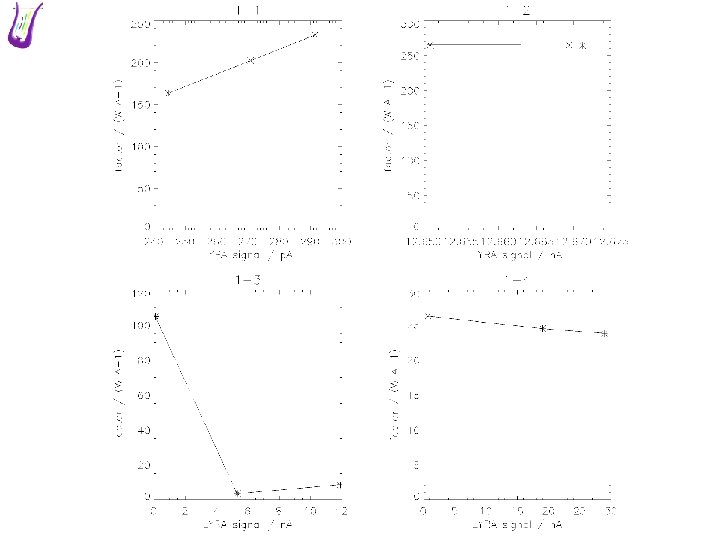
Calibration Factor, Data Levels How to estimate the solar signal from the LYRA signal? LYRA signal * purity / area / responsivity = solar signal [A] [%] [m 2] [A W-1] [W m-2] __________/ calibration factor Example: “max”, “high”, “min” flux + Channels 1 -1, 1 -2, 1 -3, 1 -4 - Use constant factor, linear dependency on signal, knowledge about solar flux? Change public data each time when calibration factor gets more realistic? Use different data levels?
 What consequences")
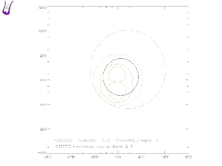
e. Homogeneity, Flatfield Example: Channel 2 -3 (detector diameter 4. 2 mm) What consequences will an off-pointing have?

f. Cadence, Response Time Example: Signal vs. integration time Channel 2 -3 (Aluminium + MSM 15) at BESSY GI 2006

III. Summary Linearity Stability LEDs Signal, Purity 1 -1 MSM 1 -2 PIN 1 -3 MSM 1 -4 AXUV + + --+ -+ + +? ? ? ++ -+++ 2 -1 MSM 2 -2 PIN 2 -3 MSM 2 -4 MSM + + -? ? ? ++ -+++ 3 -1 AXUV 3 -2 PIN 3 -3 AXUV 3 -4 AXUV + + + +? +? ? ? + ++ -+++

IV. Additional Topics - Cross-calibration Degradation of filters, detectors, LEDs Tests to be performed Normal cadence (acquisition rate) Nominal units Rate of calibration with LEDs
- Slides: 23