LYRA the LargeYield Radiometer onboard PROBA 2 LYRA

LYRA the Large-Yield Radiometer onboard PROBA 2 LYRA Calibration, Data Products, Plans I. E. Dammasch, ROB/SIDC PROBA 2 Science Meeting Sun 360, Kiel, 25 -29 Jul 2011
 n 4 spectral channels per")
LYRA: the Large-Yield RAdiometer n 3 instrument units (redundancy) n 4 spectral channels per head n 3 types of detectors, Silicon + 2 types of diamond detectors (MSM, PIN): - radiation resistant - insensitive to visible light compared to Si detectors n High cadence up to 100 Hz

SWAP and LYRA spectral intervals for solar flares, space weather, and aeronomy LYRA channel 1: the H I 121. 6 nm Lyman-alpha line (120 -123 nm) LYRA channel 2: the 200 -220 nm Herzberg continuum range (now 190 -222 nm) LYRA channel 3: the 17 -80 nm Aluminium filter range incl the He II 30. 4 nm line (+ <5 nm X-ray) LYRA channel 4: the 6 -20 nm Zirconium filter range with highest solar variablility (+ <2 nm X-ray) SWAP: the range around 17. 4 nm including coronal lines like Fe IX and Fe X
")
LYRA pre-flight spectral responsivity (filter + detector, twelve combinations)
 n Level")
Data product definition n Level 1 = full raw data (LY-EDG output) n Level 2 = calibrated physical data (LY-BSDG output) Caution: preliminary status. Require versioning. n Level 3 = processed products (e. g. averages) n Level 4 = plots of products n Level 5 = event lists (optionally with plots)
 Problems: 1. Unrealistic")
LYRA calibration … … was not as easy as anticipated (surprise!) Problems: 1. Unrealistic nominal intervals 2. Fast degradation 3. Periodically varying dark currents

Possible solutions 1. Re-define realistic nominal intervals, at least for a start 2. Estimate and correct degradation by internal means (LYRA Head 2 vs. Head 3) 3. Estimate and correct dark currents by using detector temperatures Then calibrate according to First Light Day (i. e. before degradation begins)

Most recent degradation fit

Most recent dark current fit

Observed vs. LRM-simulated values (Example: Head 2 count rates, TIMED/SEE, SORCE/SOLSTICE spectra of 06 Jan 2010) ch 2 -1 ch 2 -2 ch 2 -3 ch 2 -4 sim 0. 1030 n. A 12. 07 n. A 0. 05765 n. A 0. 1542 n. A obs 500 k. Hz dc -8. 0 k. Hz VFC, resis. => 0. 1969 n. A 710 k. Hz -6. 5 k. Hz => 14. 81 n. A 23. 0 k. Hz -6. 4 k. Hz => 0. 06780 n. A 45. 0 k. Hz -7. 5 k. Hz => 0. 1539 n. A +91. 2% +22. 8% +17. 6% -2. 0%

Resulting conversion to physical units => +81. 3% +91. 2% +3. 3% ? (0. 0%) +13. 3% +22. 8% +18. 0% => +18. 0% +11. 2% +17. 6% +11. 2% => +13. 3% +14. 3% (1) -2. 0% (2) +15. 4% (3) => +9. 2% ch*-1 ch*-2 ch*-3 ch*-4 (120 -123 nm) (190 -222 nm) (17 -80&0 -5 nm) (6 -20&0 -2 nm) 0. 006320 W/m² 0. 5914 W/m² 0. 002008 W/m² 0. 0007187 W/m² ? (0. 0%) +18. 0% +13. 3% +9. 2% => 0. 006320 W/m² 0. 6979 W/m² 0. 002275 W/m² 0. 0007848 W/m² which corresponds to. . . 492 k. Hz 703. 5 k. Hz 16. 6 k. Hz 37. 5 k. Hz (Example: Head 2, dark currents subtracted, degradation added. Simple linear conversion!)
 LYRA products … resulting from calibration attempts: n")
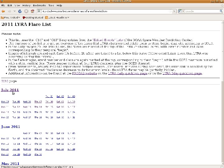
New (well, more or less new) LYRA products … resulting from calibration attempts: n Level 2 FITS files n Level 3 FITS files n (Level 4) One-day overviews n (Level 4) Three-day overviews n (Level 5) Flare lists … available here at the P 2 SC website: http: //proba 2. sidc. be/

one-day overview

three-day overview

monthly overview
")
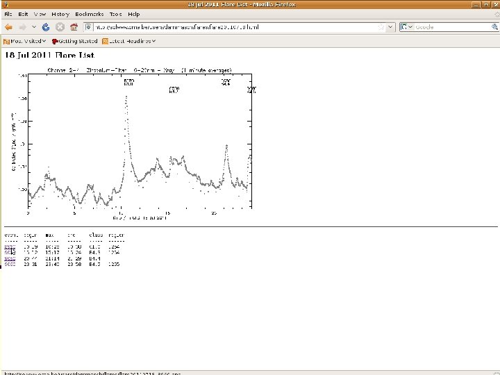
interval around a flare (-1 h, +2 h)

Jan - Sep 2010 SWAVINT and LYRA look quite similar LYRA shows flares in addition to EUV

July 2010 LYRA vs. EVE

July 2010 GOES vs. TIMED/SEE

July 2010 LYRA vs. GOES
 n LYRA observes")
LYRA flare size LYRA background-subtracted flux in Zr (channel 2 -4) n LYRA observes all GOES flares in both Al and Zr channels n Initially also Lyman-alpha contribution for impulsive flares n Different onset and peak times in different pass bands n Good correlation to GOES, better temporal resolution
 n Automating flare list n Calibration head 1, head 3 n Regular")
Plans (Routine) n Automating flare list n Calibration head 1, head 3 n Regular update of degradation n “First Light” instrument publication n Flat-field (off-pointing) effects, slow MSM-detector effects, LARs, ASICs, distance from Sun, flagging, quality factor (= old to-do-list)
 n Separate calibration EUV vs. SXR n Degradation publication (with Davos")
Plans (Special interest) n Separate calibration EUV vs. SXR n Degradation publication (with Davos team? ) n More about flares (decay time, detection, are there pure EUV flares, …)

Example

Flare components ch 2 -3 = SXR+EUV

Thank you …for your attention !

Calibration 2010 according to TIMED/SEE

Calibration – Problem: 2010 according to LYRA
 … no degradation so far …")
First Light acquisition (06 Jan 2010) … no degradation so far …

Start with “First Light”…

…estimate and subtract dark currents…

… fit the degradation …

… and add it Plausibility: - Artifacts in channels 1 and 2 - Non-degenerated SXR in channels 3 and 4 Disadvantages: - Underestimate EUV in channels 3 (and 4) - Distortion of occultations

LYRA Radiometric Model, ch 1 -1 simulated
 ch 1 -1 ch 1 -2 ch 1")
Observed vs. LRM-simulated values (head 1) ch 1 -1 ch 1 -2 ch 1 -3 ch 1 -4 sim 0. 2929 n. A 11. 28 n. A 0. 06399 n. A 0. 1064 n. A obs ~1300 k. Hz dc -9. 0 k. Hz VFC, resis. => 0. 5311 n. A 620 k. Hz -6. 6 k. Hz => 12. 78 n. A 24. 0 k. Hz -6. 8 k. Hz => 0. 07116 n. A 37. 5 k. Hz -7. 2 k. Hz => 0. 1216 n. A +81. 3% +13. 3% +11. 2% +14. 3%

LYRA Radiometric Model, ch 2 -4 simulated
 ch 2 -1 ch 2 -2 ch 2")
Observed vs. LRM-simulated values (head 2) ch 2 -1 ch 2 -2 ch 2 -3 ch 2 -4 sim 0. 1030 n. A 12. 07 n. A 0. 05765 n. A 0. 1542 n. A obs 500 k. Hz dc -8. 0 k. Hz VFC, resis. => 0. 1969 n. A 710 k. Hz -6. 5 k. Hz => 14. 81 n. A 23. 0 k. Hz -6. 4 k. Hz => 0. 06780 n. A 45. 0 k. Hz -7. 5 k. Hz => 0. 1539 n. A +91. 2% +22. 8% +17. 6% -2. 0%
 ch 3 -1 ch 3 -2 ch 3")
Observed vs. LRM-simulated values (head 3) ch 3 -1 ch 3 -2 ch 3 -3 ch 3 -4 sim 0. 3686 n. A 9. 693 n. A 1. 0250 n. A 0. 1082 n. A obs 930 k. Hz dc -10. 0 k. Hz VFC, resis. => 0. 3807 n. A 552 k. Hz -6. 5 k. Hz => 11. 44 n. A 280 k. Hz -6. 4 k. Hz => 1. 1400 n. A 36. 2 k. Hz -6. 2 k. Hz => 0. 1249 n. A +3. 3% +18. 0% +11. 2% +15. 4%
 (190 -222")
Observations by TIMED/SEE and SORCE ch*-1 ch*-2 ch*-3 ch*-4 (120 -123 nm) (190 -222 nm) (17 -80&0 -5 nm) (6 -20&0 -2 nm) 0. 006320 W/m² 0. 5914 W/m² 0. 002008 W/m² 0. 0007187 W/m² (corrected by “experts 1, 2, and 3”: ) +81. 3% +13. 3% +11. 2% +91. 2% +22. 8% +17. 6% +3. 3% +18. 0% +11. 2% => ? (0. 0%) => +18. 0% => +13. 3% +14. 3% -2. 0% +15. 4% => +9. 2% Subtract dark currents, add degradation, then 492 k. Hz 703. 5 k. Hz 16. 6 k. Hz 37. 5 k. Hz (example: head 2) is converted to. . . W/m² +. . . %

Example: Head 2, Jan 2011, before & after
 n Look plausible n Correspond")
Outlook n Samples (Jan, Apr, Sep 2010, Jan 2011) n Look plausible n Correspond with levels of other instruments n ch 2 -3 and ch 2 -4 correspond with variation structure of other instruments n Flares (SXR) are probably overestimated n TBD: flat-field (off-pointing) effects, slow MSMdetector effects, LARs, ASICs, distance from Sun, flagging, quality factor n Suggestions ?
- Slides: 45