LSP 121 Week 2 Intro to Statistics and

LSP 121 Week 2 Intro to Statistics and SPSS/PASW

Descriptive Statistics: Mean, Median, Percentile, Range • Mean • Median – the middle score • The score with an equal number of data points above and below • If there an even number of datapoints, take the average of the middle two • Percent Rank – calculates the position of a datapoint in a data set. More precisely, tells you approximately how many percent of the data is less than the datapoint. • e. g. 86 th percentile means that 86 percent of data-points /people / etc were below that number • Range – difference between the maximum and minimum values in the data set 2

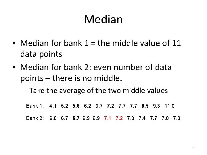
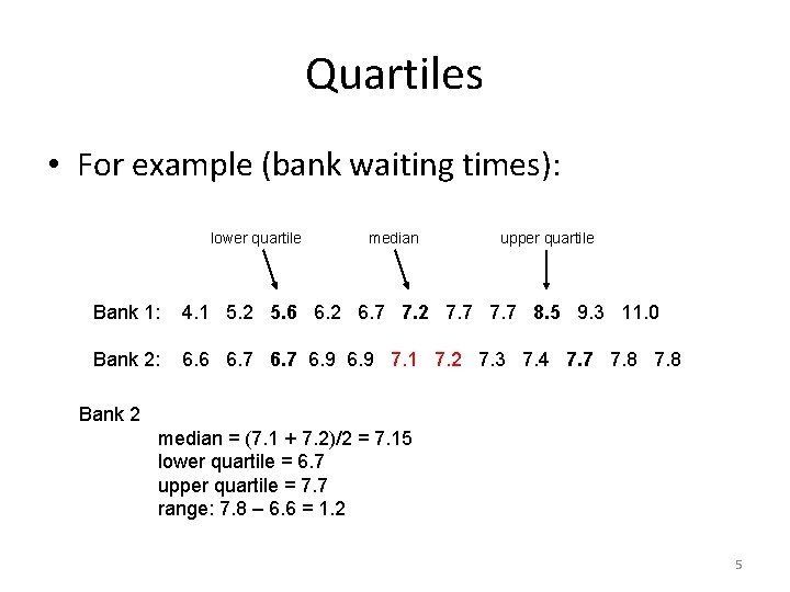
Median • Median for bank 1 = the middle value of 11 data points • Median for bank 2: even number of data points – there is no middle. – Take the average of the two middle values Bank 1: 4. 1 5. 2 5. 6 6. 2 6. 7 7. 2 7. 7 8. 5 9. 3 11. 0 Bank 2: 6. 6 6. 7 6. 9 7. 1 7. 2 7. 3 7. 4 7. 7 7. 8 3

Descriptive Statistics: Quartiles • Lower quartile: aka first quartile - the median of the data values in the lower half of a data set (do not include the median) • Middle quartile: aka second quartile - this is the overall median • Upper quartile: aka third quartile - the median of the data values in the upper half of a data set (do not include the median) – Note: Some statistical software packages use the 25 th, 50 th, and 75 th percentiles as their quartiles (instead of median values). SPSS determines quartiles in this way. On an exam, you would use the medians. 4

Quartiles • For example (bank waiting times): lower quartile median upper quartile Bank 1: 4. 1 5. 2 5. 6 6. 2 6. 7 7. 2 7. 7 8. 5 9. 3 11. 0 Bank 2: 6. 6 6. 7 6. 9 7. 1 7. 2 7. 3 7. 4 7. 7 7. 8 Bank 2 median = (7. 1 + 7. 2)/2 = 7. 15 lower quartile = 6. 7 upper quartile = 7. 7 range: 7. 8 – 6. 6 = 1. 2 5

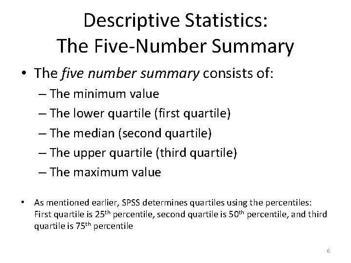
Descriptive Statistics: The Five-Number Summary • The five number summary consists of: – The minimum value – The lower quartile (first quartile) – The median (second quartile) – The upper quartile (third quartile) – The maximum value • As mentioned earlier, SPSS determines quartiles using the percentiles: First quartile is 25 th percentile, second quartile is 50 th percentile, and third quartile is 75 th percentile 6

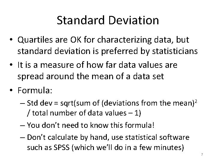
Standard Deviation • Quartiles are OK for characterizing data, but standard deviation is preferred by statisticians • It is a measure of how far data values are spread around the mean of a data set • Formula: – Std dev = sqrt(sum of (deviations from the mean)2 / total number of data values – 1) – You don’t need to know this formula! – Don’t calculate by hand, use statistical software such as SPSS (which we’ll do in a few minutes) 7

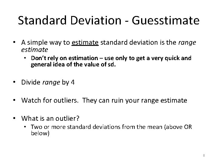
Standard Deviation - Guesstimate • A simple way to estimate standard deviation is the range estimate • Don’t rely on estimation – use only to get a very quick and general idea of the value of sd. • Divide range by 4 • Watch for outliers. They can ruin your range estimate • What is an outlier? • Two or more standard deviations from the mean (above OR below) 8

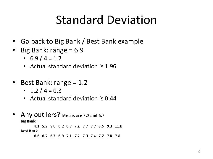
Standard Deviation • Go back to Big Bank / Best Bank example • Big Bank: range = 6. 9 • 6. 9 / 4 = 1. 7 • Actual standard deviation is 1. 96 • Best Bank: range = 1. 2 • 1. 2 / 4 = 0. 3 • Actual standard deviation is 0. 44 • Any outliers? Means are 7. 2 and 6. 7 Big Bank: 4. 1 5. 2 5. 6 6. 2 6. 7 7. 2 7. 7 8. 5 9. 3 11. 0 Best Bank: 6. 6 6. 7 6. 9 7. 1 7. 2 7. 3 7. 4 7. 7 7. 8 9

* Histograms • Nice way to view a data set • A histogram is a chart created by defining a set of bins and counting how many data points lie in each bin. Bars are drawn with height proportional to the number of data points in each bin. – * Note: The histogram does not keep track of the value of each data point – it only keeps track of which bin a data point is contained in. 10

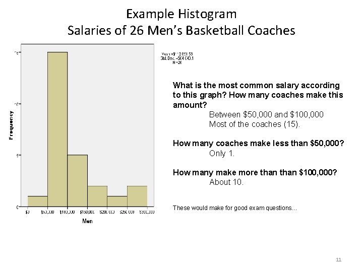
Example Histogram Salaries of 26 Men’s Basketball Coaches What is the most common salary according to this graph? How many coaches make this amount? Between $50, 000 and $100, 000 Most of the coaches (15). How many coaches make less than $50, 000? Only 1. How many make more than $100, 000? About 10. These would make for good exam questions… 11

Statistics and SPSS/PASW • While Excel can do some basic statistics, it is not considered a serious statistics tool • You really should use something like SPSS/PASW or SAS • We’ll use SPSS/PASW since De. Paul has a site license 12

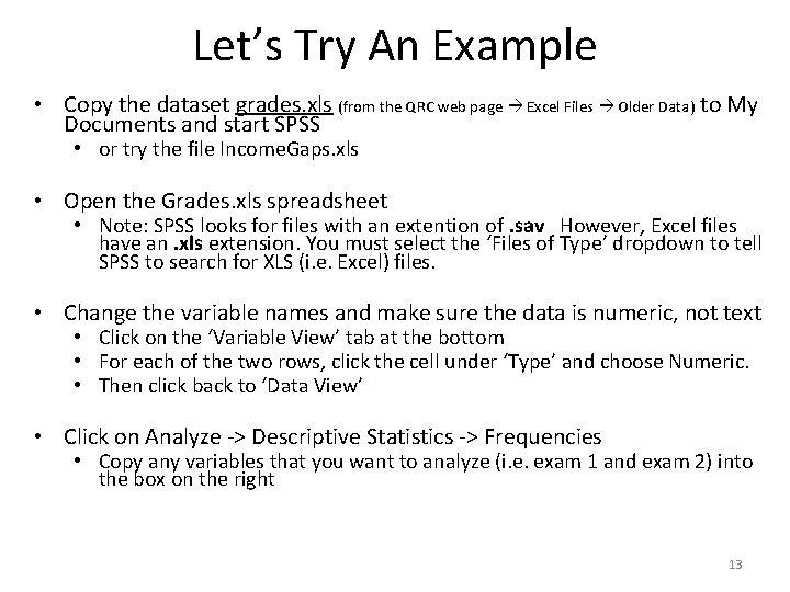
Let’s Try An Example • Copy the dataset grades. xls (from the QRC web page Excel Files Older Data) to My Documents and start SPSS • or try the file Income. Gaps. xls • Open the Grades. xls spreadsheet • Note: SPSS looks for files with an extention of. sav However, Excel files have an. xls extension. You must select the ‘Files of Type’ dropdown to tell SPSS to search for XLS (i. e. Excel) files. • Change the variable names and make sure the data is numeric, not text • Click on the ‘Variable View’ tab at the bottom • For each of the two rows, click the cell under ‘Type’ and choose Numeric. • Then click back to ‘Data View’ • Click on Analyze -> Descriptive Statistics -> Frequencies • Copy any variables that you want to analyze (i. e. exam 1 and exam 2) into the box on the right 13

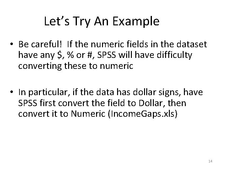
Let’s Try An Example • Be careful! If the numeric fields in the dataset have any $, % or #, SPSS will have difficulty converting these to numeric • In particular, if the data has dollar signs, have SPSS first convert the field to Dollar, then convert it to Numeric (Income. Gaps. xls) 14

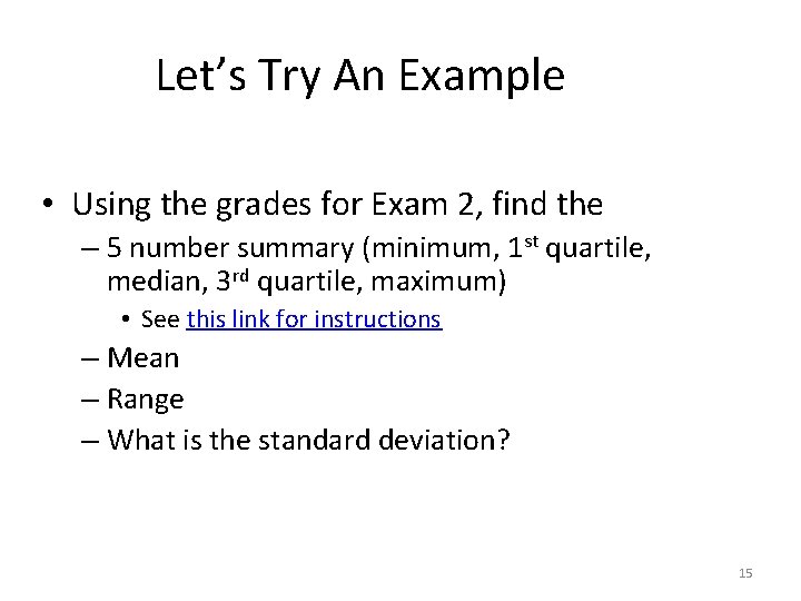
Let’s Try An Example • Using the grades for Exam 2, find the – 5 number summary (minimum, 1 st quartile, median, 3 rd quartile, maximum) • See this link for instructions – Mean – Range – What is the standard deviation? 15

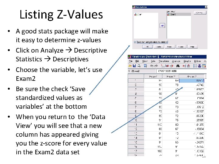
Listing Z-Values • A good stats package will make it easy to determine z-values • Click on Analyze Descriptive Statistics Descriptives • Choose the variable, let’s use Exam 2 • Be sure the check ‘Save standardized values as variables’ at the bottom • When you return to the ‘Data View’ you will see that a new column has appeared giving you the z-score for every value in the Exam 2 data set 16

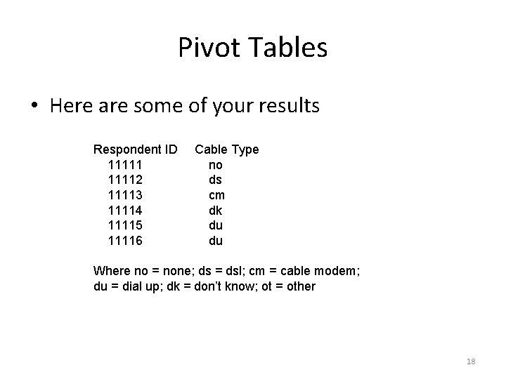
Pivot Tables • Let’s say you have just performed a survey. • One of the questions you ask is: “What type of home computer Internet connection do you have? ” – Answers can be: None, Dial-up, DSL, Cable, Other, Not Sure. 17

Pivot Tables • Here are some of your results Respondent ID 111112 11113 11114 11115 11116 Cable Type no ds cm dk du du Where no = none; ds = dsl; cm = cable modem; du = dial up; dk = don’t know; ot = other 18

Pivot Tables • You can use SPSS to count the occurrences of data items, just like a pivot table • Open a new file: File New • Enter your data into SPSS (you can leave out the IDs for now) • Click on Analyze / Descriptive Statistics / Frequencies • Move the variable that you want to count from the left box to the right box • Make sure Display Frequencies Table is checked • Run it (Click ‘OK’) 19

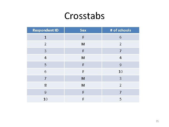
Crosstabulations (Crosstabs) • Crosstabs are an extension of pivot tables • Let’s say you have asked a number of students: How many schools did you apply to? • You get results something like the following (in a spreadsheet): 20

Crosstabs Respondent ID Sex # of schools 1 F 6 2 M 2 3 F 7 4 M 4 5 F 9 6 F 10 7 M 3 8 M 2 9 F 7 10 F 5 21

Crosstabs • Now open the data in SPSS • Then pull down the menu Analyze and click on Descriptive Statistics, then Crosstabs • What variable do you want in the row? The column? – We are probably interested in determining examining how many schools females apply to relative to males • When ready, click OK to perform the crosstab. 22