LSA 352 Speech Recognition and Synthesis Dan Jurafsky

LSA 352 Speech Recognition and Synthesis Dan Jurafsky Lecture 6: Feature Extraction and Acoustic Modeling IP Notice: Various slides were derived from Andrew Ng’s CS 229 notes, as well as lecture notes from Chen, Picheny et al, Yun-Hsuan Sung, and Bryan Pellom. I’ll try to give correct credit on each slide, but I’ll prob miss some. LSA 352 Summer 2007 1

Outline for Today Feature Extraction (MFCCs) The Acoustic Model: Gaussian Mixture Models (GMMs) Evaluation (Word Error Rate) How this fits into the ASR component of course July 6: Language Modeling July 19: HMMs, Forward, Viterbi, July 23: Feature Extraction, MFCCs, Gaussian Acoustic modeling, and hopefully Evaluation July 26: Spillover, Baum-Welch (EM) training LSA 352 Summer 2007 2

Outline for Today Feature Extraction Mel-Frequency Cepstral Coefficients Acoustic Model Increasingly sophisticated models Acoustic Likelihood for each state: – Gaussians – Multivariate Gaussians – Mixtures of Multivariate Gaussians Where a state is progressively: – CI Subphone (3 ish per phone) – CD phone (=triphones) – State-tying of CD phone Evaluation Word Error Rate LSA 352 Summer 2007 3

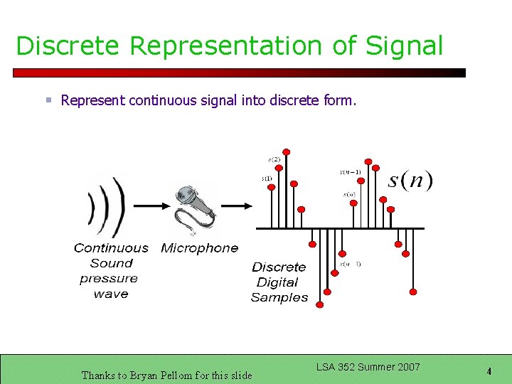
Discrete Representation of Signal Represent continuous signal into discrete form. Thanks to Bryan Pellom for this slide LSA 352 Summer 2007 4

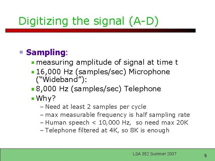
Digitizing the signal (A-D) Sampling: measuring amplitude of signal at time t 16, 000 Hz (samples/sec) Microphone (“Wideband”): 8, 000 Hz (samples/sec) Telephone Why? – Need at least 2 samples per cycle – max measurable frequency is half sampling rate – Human speech < 10, 000 Hz, so need max 20 K – Telephone filtered at 4 K, so 8 K is enough LSA 352 Summer 2007 5

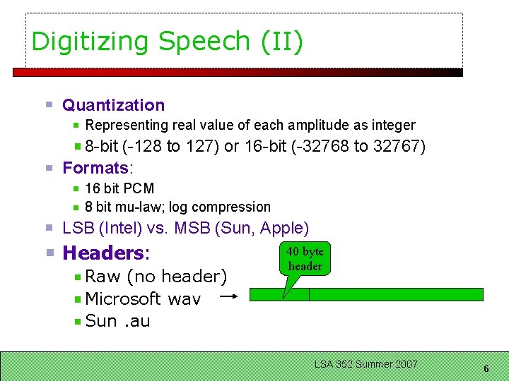
Digitizing Speech (II) Quantization Representing real value of each amplitude as integer 8 -bit (-128 to 127) or 16 -bit (-32768 to 32767) Formats: 16 bit PCM 8 bit mu-law; log compression LSB (Intel) vs. MSB (Sun, Apple) Headers: Raw (no header) Microsoft wav Sun. au 40 byte header LSA 352 Summer 2007 6

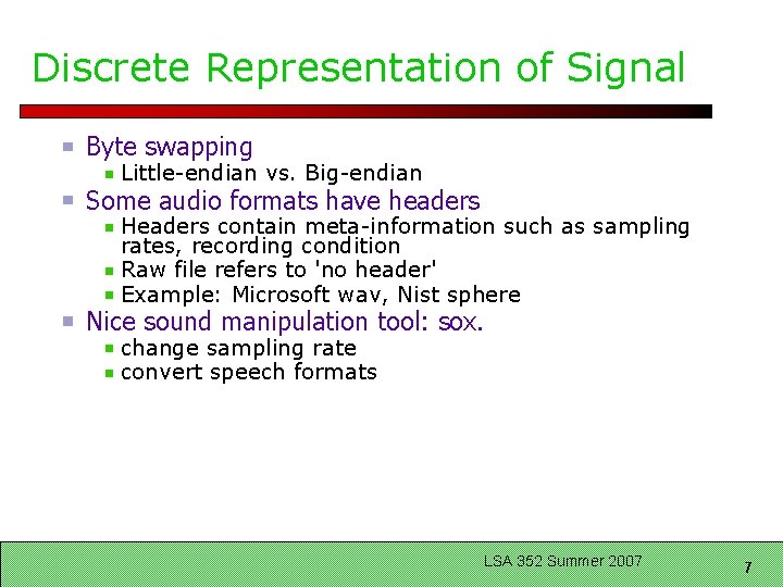
Discrete Representation of Signal Byte swapping Little-endian vs. Big-endian Some audio formats have headers Headers contain meta-information such as sampling rates, recording condition Raw file refers to 'no header' Example: Microsoft wav, Nist sphere Nice sound manipulation tool: sox. change sampling rate convert speech formats LSA 352 Summer 2007 7

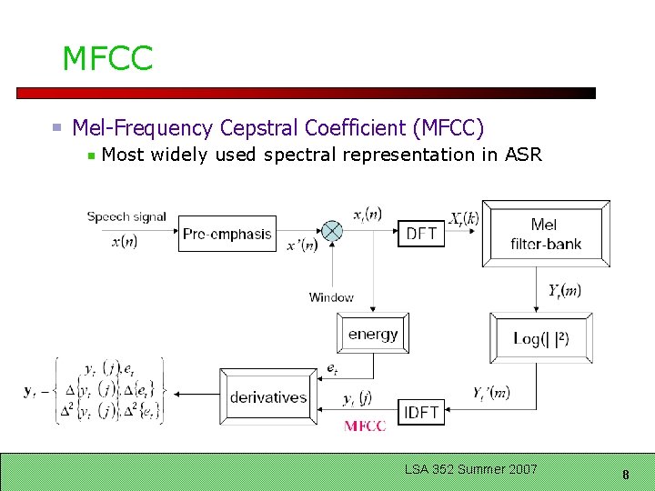
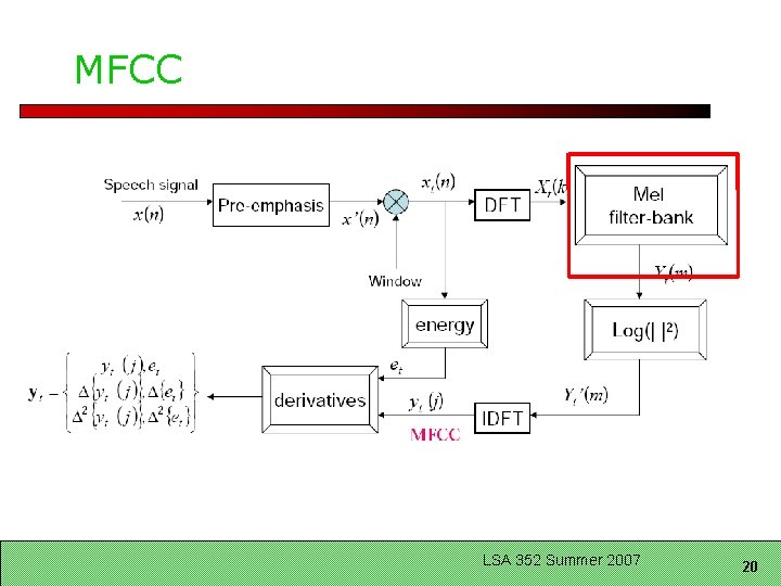
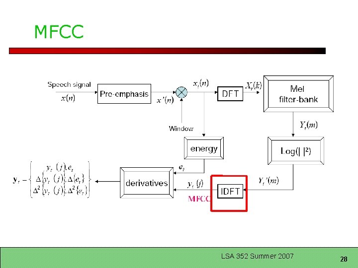
MFCC Mel-Frequency Cepstral Coefficient (MFCC) Most widely used spectral representation in ASR LSA 352 Summer 2007 8

Pre-Emphasis Pre-emphasis: boosting the energy in the high frequencies Q: Why do this? A: The spectrum for voiced segments has more energy at lower frequencies than higher frequencies. This is called spectral tilt Spectral tilt is caused by the nature of the glottal pulse Boosting high-frequency energy gives more info to Acoustic Model Improves phone recognition performance LSA 352 Summer 2007 9

Example of pre-emphasis Before and after pre-emphasis Spectral slice from the vowel [aa] LSA 352 Summer 2007 10

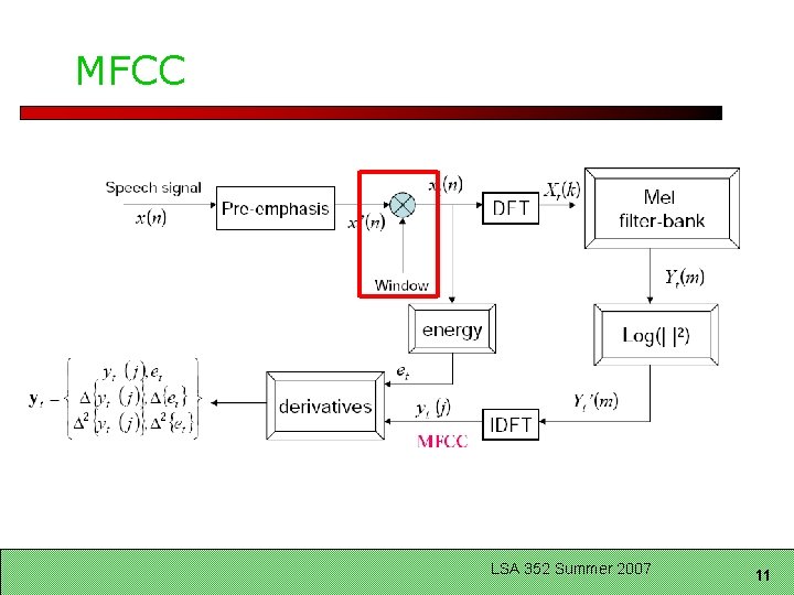
MFCC LSA 352 Summer 2007 11

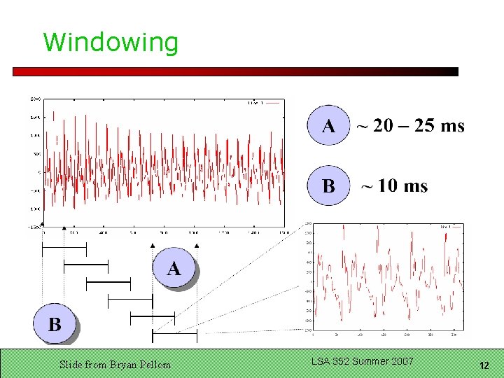
Windowing Slide from Bryan Pellom LSA 352 Summer 2007 12

Windowing Why divide speech signal into successive overlapping frames? Speech is not a stationary signal; we want information about a small enough region that the spectral information is a useful cue. Frames Frame size: typically, 10 -25 ms Frame shift: the length of time between successive frames, typically, 5 -10 ms LSA 352 Summer 2007 13

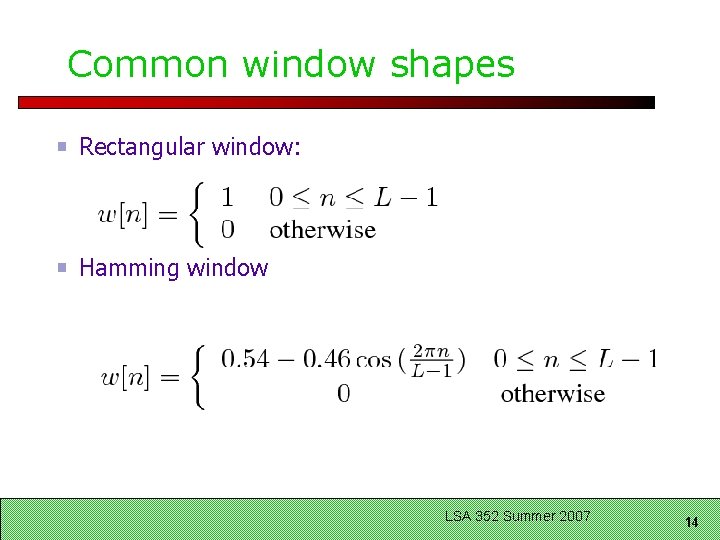
Common window shapes Rectangular window: Hamming window LSA 352 Summer 2007 14

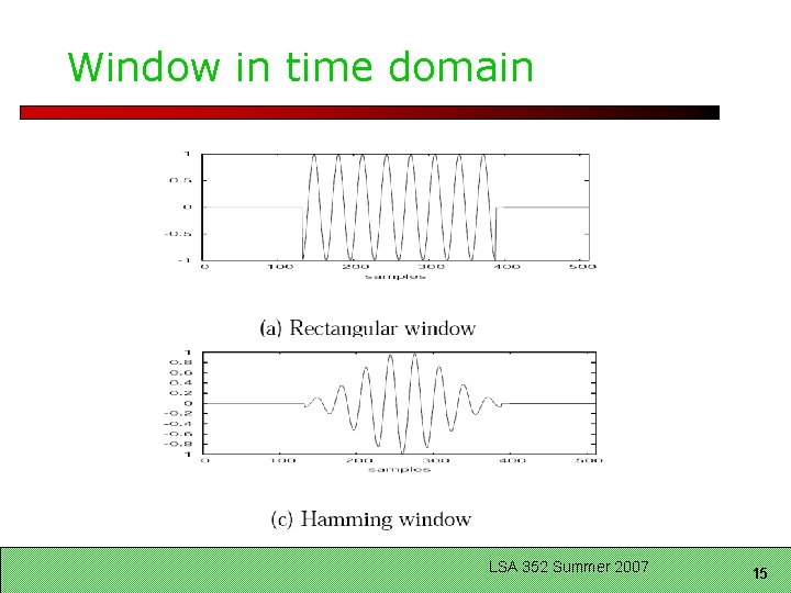
Window in time domain LSA 352 Summer 2007 15

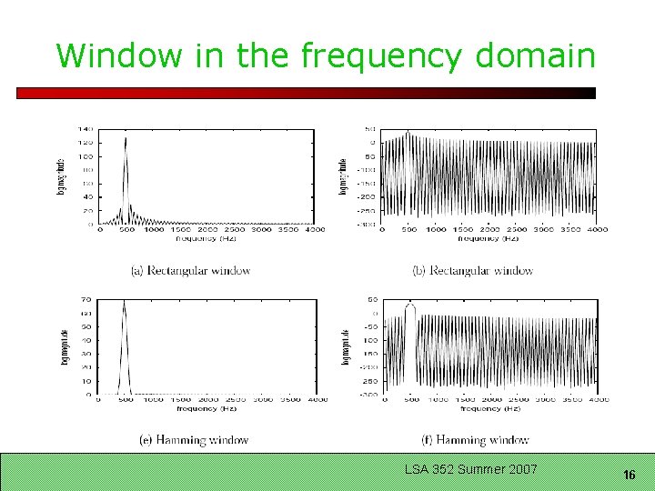
Window in the frequency domain LSA 352 Summer 2007 16

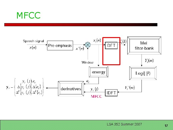
MFCC LSA 352 Summer 2007 17

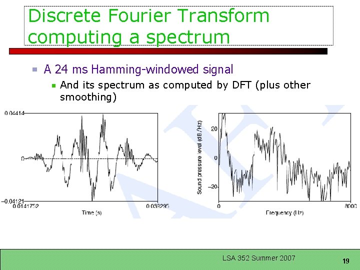
Discrete Fourier Transform Input: Windowed signal x[n]…x[m] Output: For each of N discrete frequency bands A complex number X[k] representing magnidue and phase of that frequency component in the original signal Discrete Fourier Transform (DFT) Standard algorithm for computing DFT: Fast Fourier Transform (FFT) with complexity N*log(N) In general, choose N=512 or 1024 LSA 352 Summer 2007 18

Discrete Fourier Transform computing a spectrum A 24 ms Hamming-windowed signal And its spectrum as computed by DFT (plus other smoothing) LSA 352 Summer 2007 19

MFCC LSA 352 Summer 2007 20

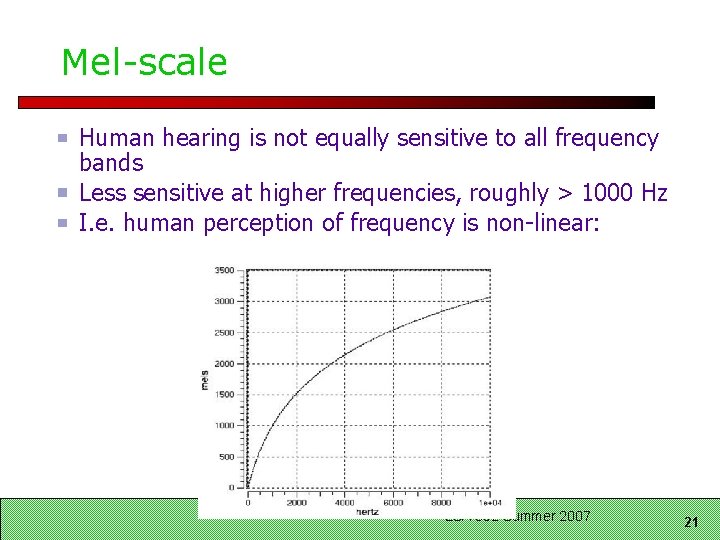
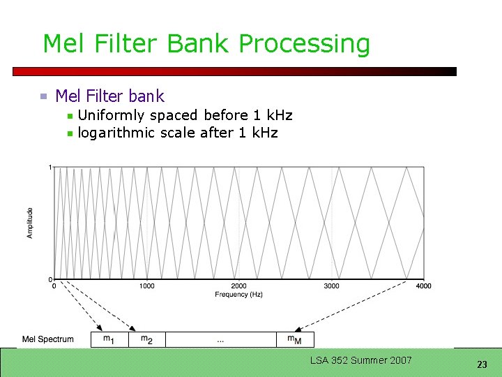
Mel-scale Human hearing is not equally sensitive to all frequency bands Less sensitive at higher frequencies, roughly > 1000 Hz I. e. human perception of frequency is non-linear: LSA 352 Summer 2007 21

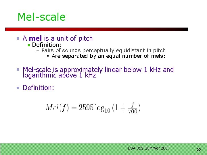
Mel-scale A mel is a unit of pitch Definition: – Pairs of sounds perceptually equidistant in pitch § Are separated by an equal number of mels: Mel-scale is approximately linear below 1 k. Hz and logarithmic above 1 k. Hz Definition: LSA 352 Summer 2007 22

Mel Filter Bank Processing Mel Filter bank Uniformly spaced before 1 k. Hz logarithmic scale after 1 k. Hz LSA 352 Summer 2007 23

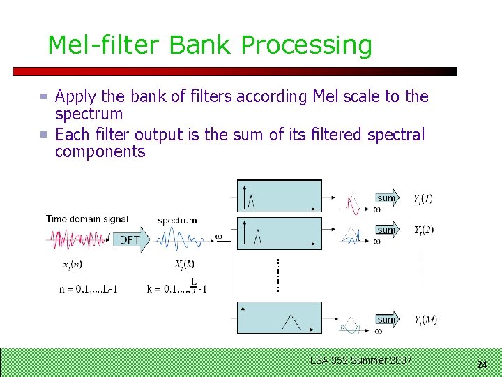
Mel-filter Bank Processing Apply the bank of filters according Mel scale to the spectrum Each filter output is the sum of its filtered spectral components LSA 352 Summer 2007 24

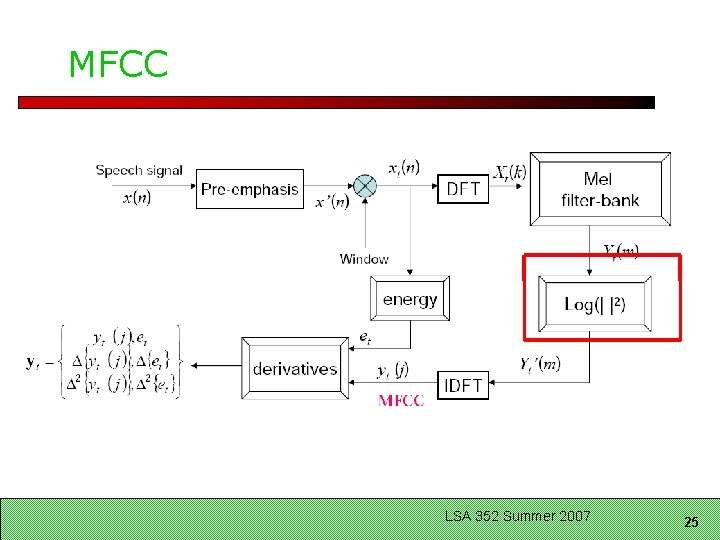
MFCC LSA 352 Summer 2007 25

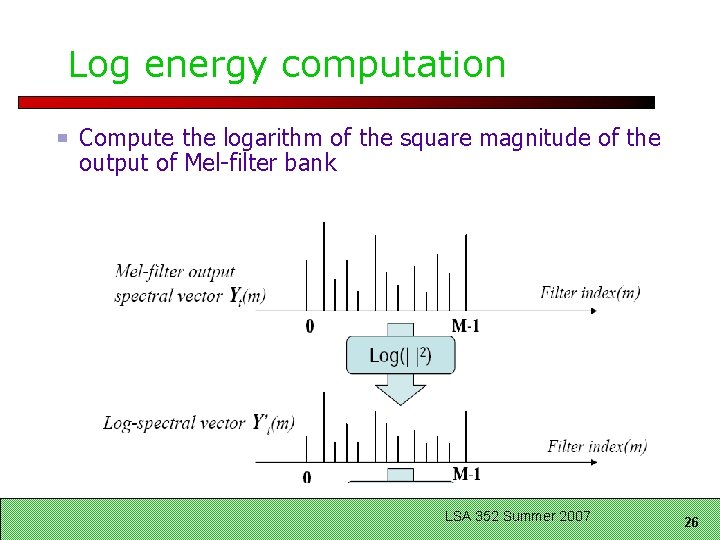
Log energy computation Compute the logarithm of the square magnitude of the output of Mel-filter bank LSA 352 Summer 2007 26

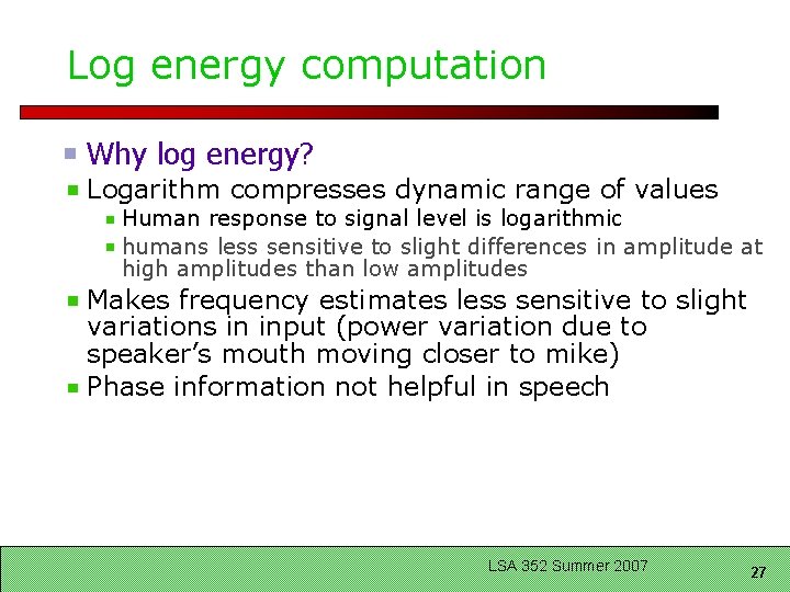
Log energy computation Why log energy? Logarithm compresses dynamic range of values Human response to signal level is logarithmic humans less sensitive to slight differences in amplitude at high amplitudes than low amplitudes Makes frequency estimates less sensitive to slight variations in input (power variation due to speaker’s mouth moving closer to mike) Phase information not helpful in speech LSA 352 Summer 2007 27

MFCC LSA 352 Summer 2007 28

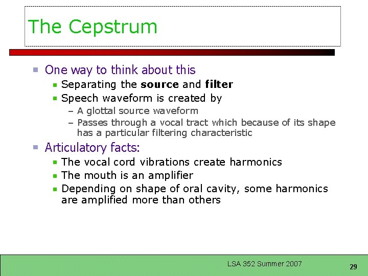
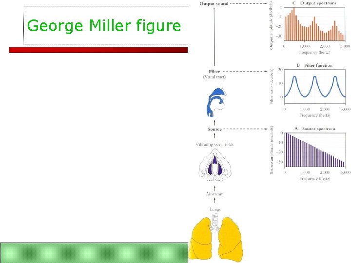
The Cepstrum One way to think about this Separating the source and filter Speech waveform is created by – A glottal source waveform – Passes through a vocal tract which because of its shape has a particular filtering characteristic Articulatory facts: The vocal cord vibrations create harmonics The mouth is an amplifier Depending on shape of oral cavity, some harmonics are amplified more than others LSA 352 Summer 2007 29

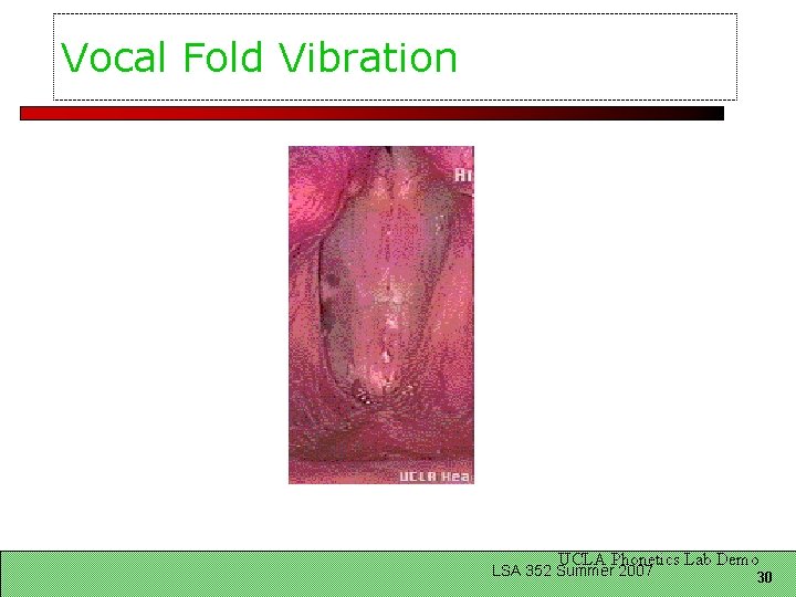
Vocal Fold Vibration UCLA Phonetics Lab Demo LSA 352 Summer 2007 30

George Miller figure LSA 352 Summer 2007 31

We care about the filter not the source Most characteristics of the source F 0 Details of glottal pulse Don’t matter for phone detection What we care about is the filter The exact position of the articulators in the oral tract So we want a way to separate these And use only the filter function LSA 352 Summer 2007 32

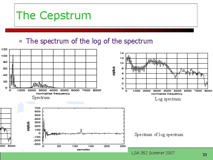
The Cepstrum The spectrum of the log of the spectrum Spectrum Log spectrum Spectrum of log spectrum LSA 352 Summer 2007 33

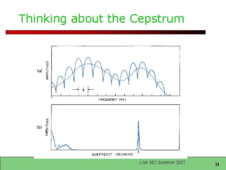
Thinking about the Cepstrum LSA 352 Summer 2007 34

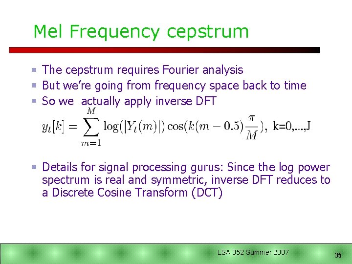
Mel Frequency cepstrum The cepstrum requires Fourier analysis But we’re going from frequency space back to time So we actually apply inverse DFT Details for signal processing gurus: Since the log power spectrum is real and symmetric, inverse DFT reduces to a Discrete Cosine Transform (DCT) LSA 352 Summer 2007 35

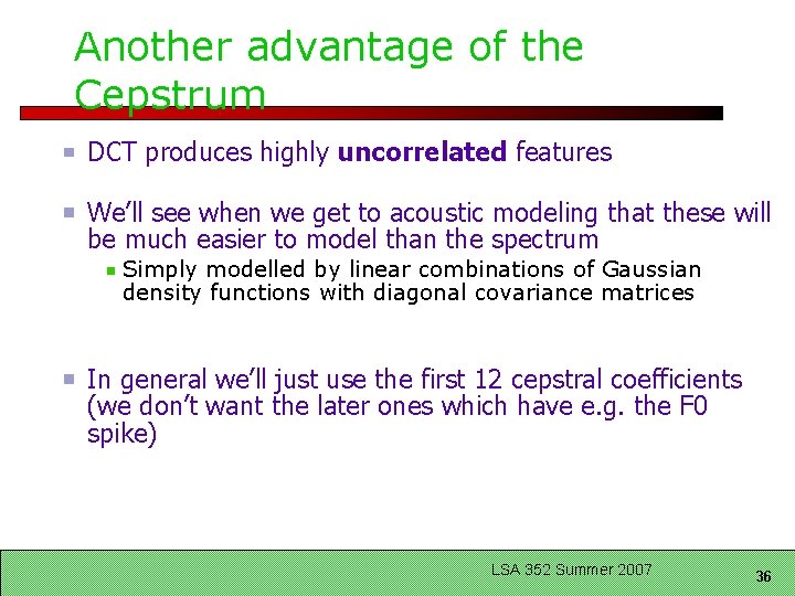
Another advantage of the Cepstrum DCT produces highly uncorrelated features We’ll see when we get to acoustic modeling that these will be much easier to model than the spectrum Simply modelled by linear combinations of Gaussian density functions with diagonal covariance matrices In general we’ll just use the first 12 cepstral coefficients (we don’t want the later ones which have e. g. the F 0 spike) LSA 352 Summer 2007 36

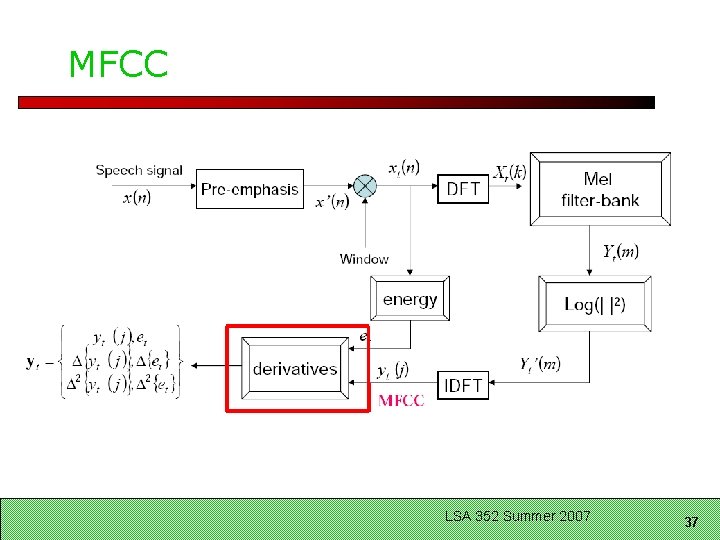
MFCC LSA 352 Summer 2007 37

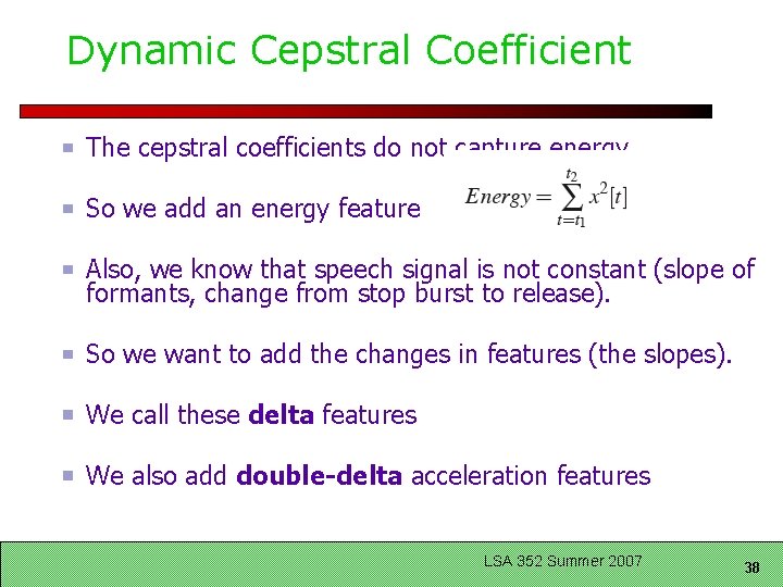
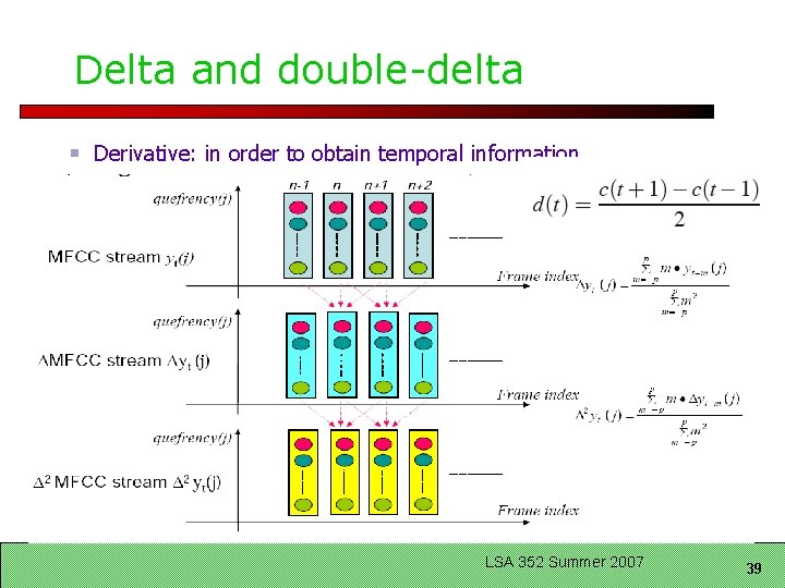
Dynamic Cepstral Coefficient The cepstral coefficients do not capture energy So we add an energy feature Also, we know that speech signal is not constant (slope of formants, change from stop burst to release). So we want to add the changes in features (the slopes). We call these delta features We also add double-delta acceleration features LSA 352 Summer 2007 38

Delta and double-delta Derivative: in order to obtain temporal information LSA 352 Summer 2007 39

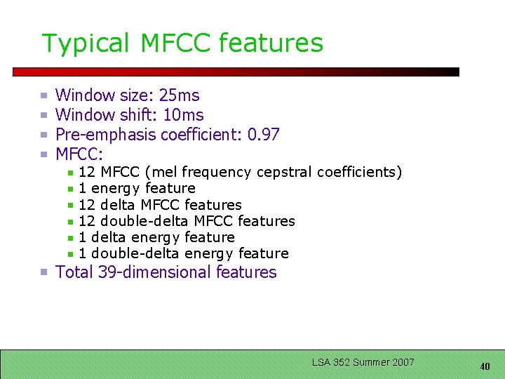
Typical MFCC features Window size: 25 ms Window shift: 10 ms Pre-emphasis coefficient: 0. 97 MFCC: 12 MFCC (mel frequency cepstral coefficients) 1 energy feature 12 delta MFCC features 12 double-delta MFCC features 1 delta energy feature 1 double-delta energy feature Total 39 -dimensional features LSA 352 Summer 2007 40

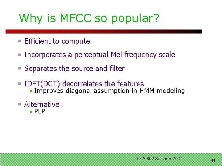
Why is MFCC so popular? Efficient to compute Incorporates a perceptual Mel frequency scale Separates the source and filter IDFT(DCT) decorrelates the features Improves diagonal assumption in HMM modeling Alternative PLP LSA 352 Summer 2007 41

Now on to Acoustic Modeling LSA 352 Summer 2007 42

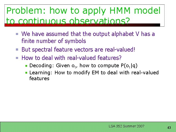
Problem: how to apply HMM model to continuous observations? We have assumed that the output alphabet V has a finite number of symbols But spectral feature vectors are real-valued! How to deal with real-valued features? Decoding: Given ot, how to compute P(ot|q) Learning: How to modify EM to deal with real-valued features LSA 352 Summer 2007 43

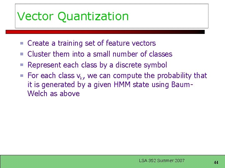
Vector Quantization Create a training set of feature vectors Cluster them into a small number of classes Represent each class by a discrete symbol For each class vk, we can compute the probability that it is generated by a given HMM state using Baum. Welch as above LSA 352 Summer 2007 44

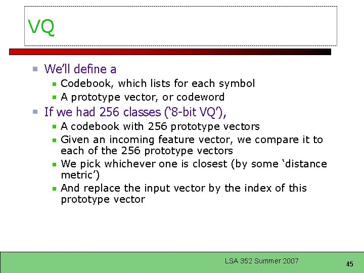
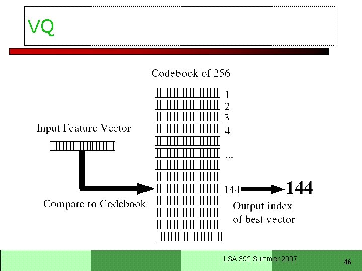
VQ We’ll define a Codebook, which lists for each symbol A prototype vector, or codeword If we had 256 classes (‘ 8 -bit VQ’), A codebook with 256 prototype vectors Given an incoming feature vector, we compare it to each of the 256 prototype vectors We pick whichever one is closest (by some ‘distance metric’) And replace the input vector by the index of this prototype vector LSA 352 Summer 2007 45

VQ LSA 352 Summer 2007 46

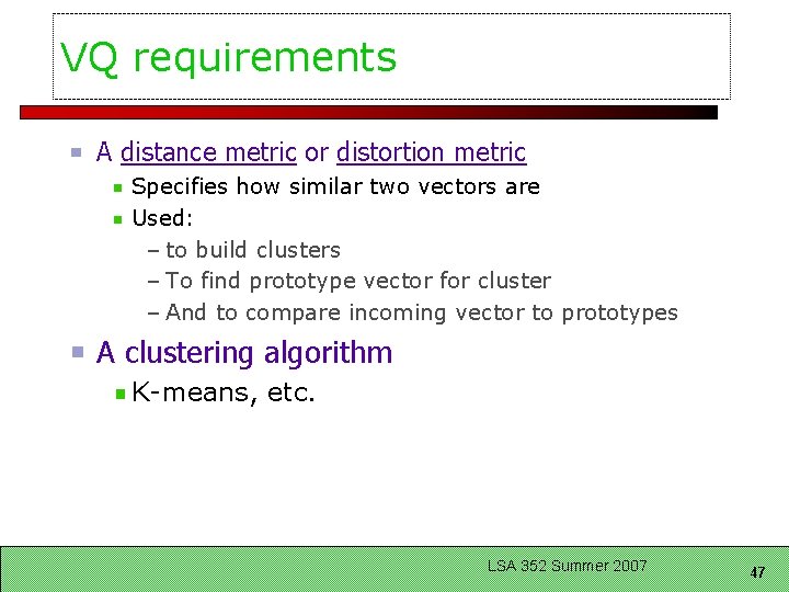
VQ requirements A distance metric or distortion metric Specifies how similar two vectors are Used: – to build clusters – To find prototype vector for cluster – And to compare incoming vector to prototypes A clustering algorithm K-means, etc. LSA 352 Summer 2007 47

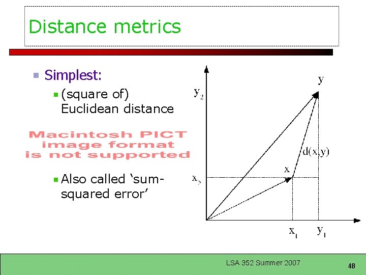
Distance metrics Simplest: (square of) Euclidean distance Also called ‘sumsquared error’ LSA 352 Summer 2007 48

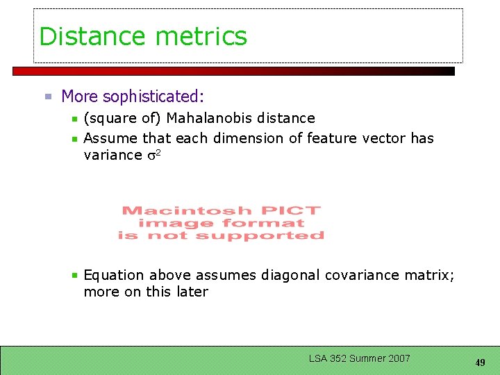
Distance metrics More sophisticated: (square of) Mahalanobis distance Assume that each dimension of feature vector has variance 2 Equation above assumes diagonal covariance matrix; more on this later LSA 352 Summer 2007 49

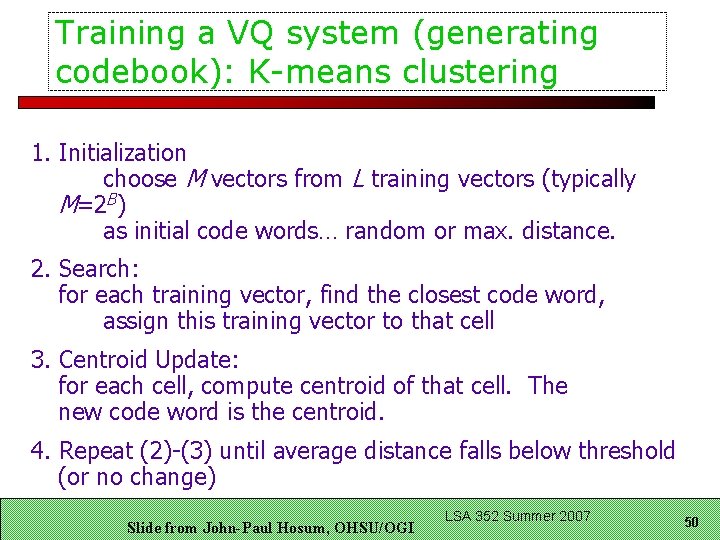
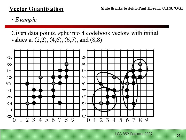
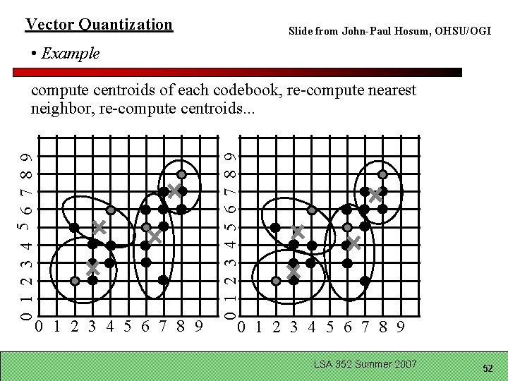
Training a VQ system (generating codebook): K-means clustering 1. Initialization choose M vectors from L training vectors (typically M=2 B) as initial code words… random or max. distance. 2. Search: for each training vector, find the closest code word, assign this training vector to that cell 3. Centroid Update: for each cell, compute centroid of that cell. The new code word is the centroid. 4. Repeat (2)-(3) until average distance falls below threshold (or no change) Slide from John-Paul Hosum, OHSU/OGI LSA 352 Summer 2007 50

Vector Quantization Slide thanks to John-Paul Hosum, OHSU/OGI • Example 0 1 2 3 4 5 6 7 8 9 Given data points, split into 4 codebook vectors with initial values at (2, 2), (4, 6), (6, 5), and (8, 8) 0 1 2 3 4 5 6 7 8 9 LSA 352 Summer 2007 51

Vector Quantization Slide from John-Paul Hosum, OHSU/OGI • Example 0 1 2 3 4 5 6 7 8 9 compute centroids of each codebook, re-compute nearest neighbor, re-compute centroids. . . 0 1 2 3 4 5 6 7 8 9 LSA 352 Summer 2007 52

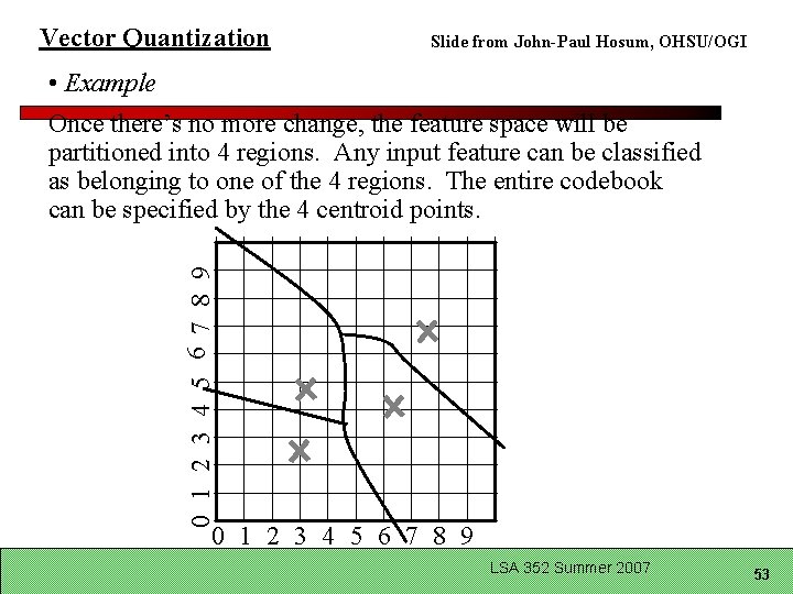
Vector Quantization Slide from John-Paul Hosum, OHSU/OGI 0 1 2 3 4 5 6 7 8 9 • Example Once there’s no more change, the feature space will be partitioned into 4 regions. Any input feature can be classified as belonging to one of the 4 regions. The entire codebook can be specified by the 4 centroid points. 0 1 2 3 4 5 6 7 8 9 LSA 352 Summer 2007 53

Summary: VQ To compute p(ot|qj) Compute distance between feature vector ot – and each codeword (prototype vector) – in a preclustered codebook – where distance is either § Euclidean § Mahalanobis Choose the vector that is the closest to ot – and take its codeword vk And then look up the likelihood of vk given HMM state j in the B matrix Bj(ot)=bj(vk) s. t. vk is codeword of closest vector to ot Using Baum-Welch as above LSA 352 Summer 2007 54

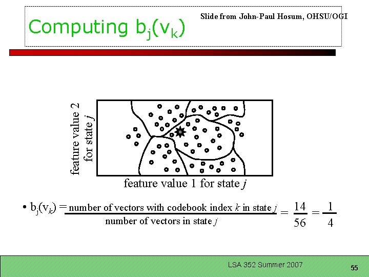
feature value 2 for state j Computing bj(vk) Slide from John-Paul Hosum, OHSU/OGI feature value 1 for state j • bj(vk) = number of vectors with codebook index k in state j = 14 = 1 number of vectors in state j 56 4 LSA 352 Summer 2007 55

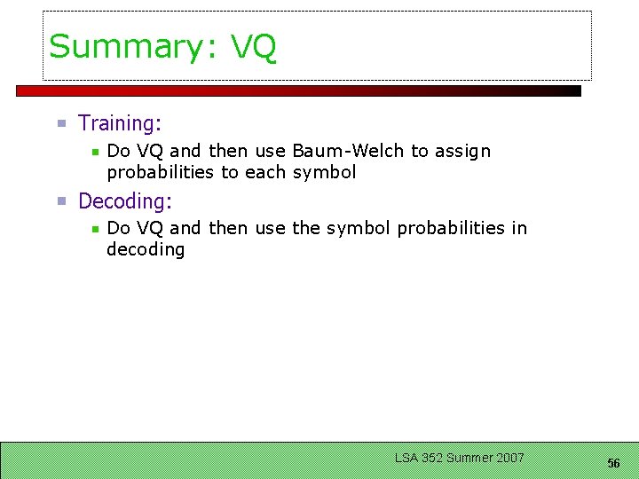
Summary: VQ Training: Do VQ and then use Baum-Welch to assign probabilities to each symbol Decoding: Do VQ and then use the symbol probabilities in decoding LSA 352 Summer 2007 56

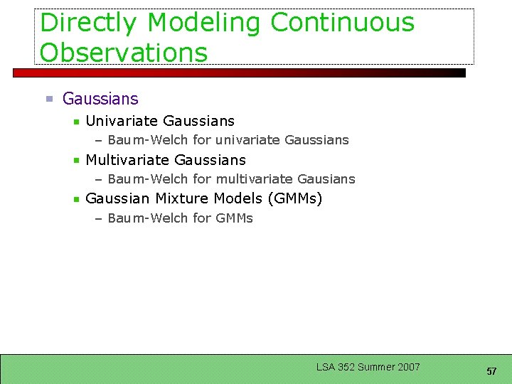
Directly Modeling Continuous Observations Gaussians Univariate Gaussians – Baum-Welch for univariate Gaussians Multivariate Gaussians – Baum-Welch for multivariate Gausians Gaussian Mixture Models (GMMs) – Baum-Welch for GMMs LSA 352 Summer 2007 57

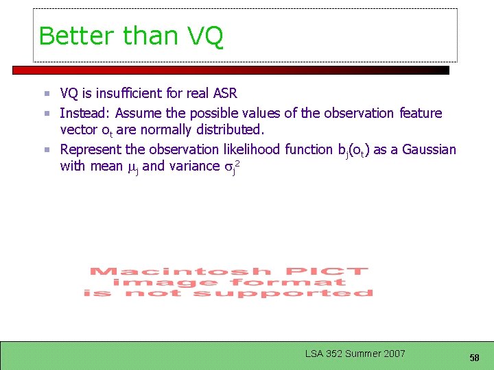
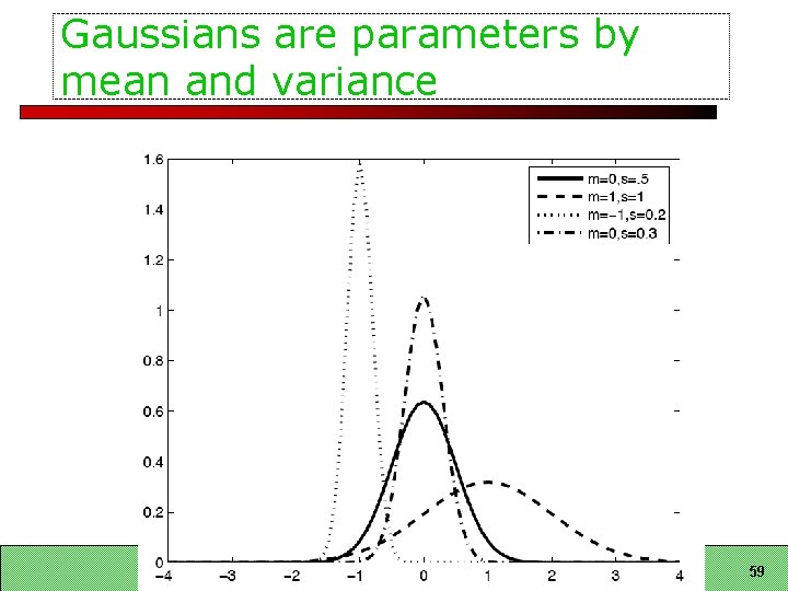
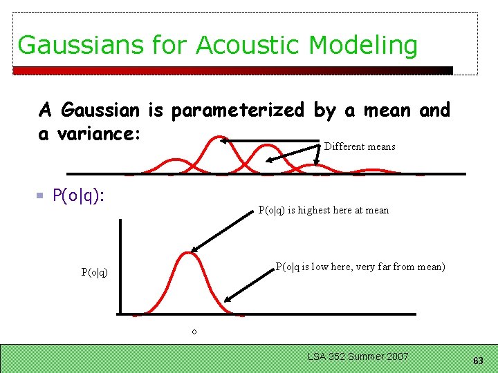
Better than VQ VQ is insufficient for real ASR Instead: Assume the possible values of the observation feature vector ot are normally distributed. Represent the observation likelihood function bj(ot) as a Gaussian with mean j and variance j 2 LSA 352 Summer 2007 58

Gaussians are parameters by mean and variance LSA 352 Summer 2007 59

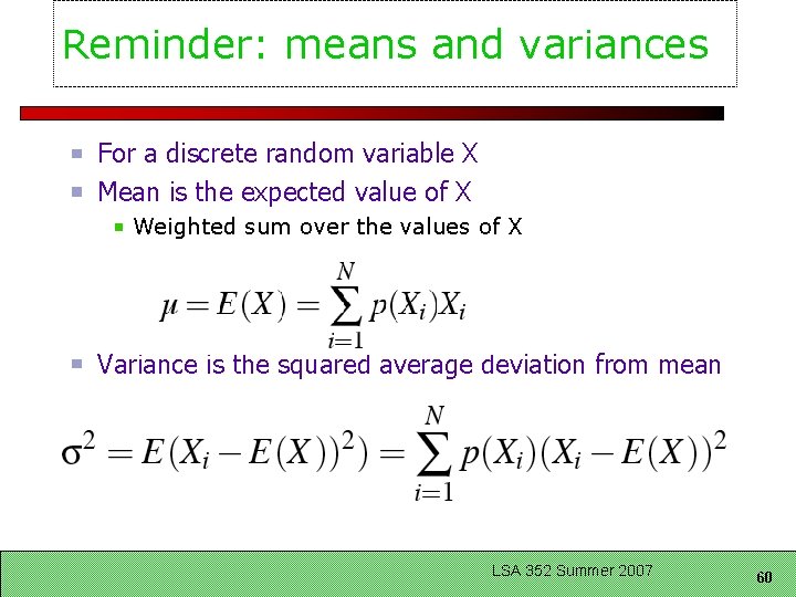
Reminder: means and variances For a discrete random variable X Mean is the expected value of X Weighted sum over the values of X Variance is the squared average deviation from mean LSA 352 Summer 2007 60

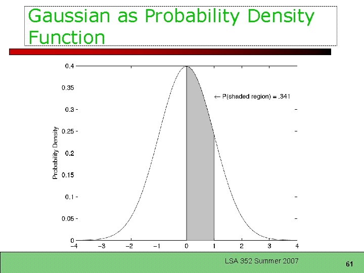
Gaussian as Probability Density Function LSA 352 Summer 2007 61

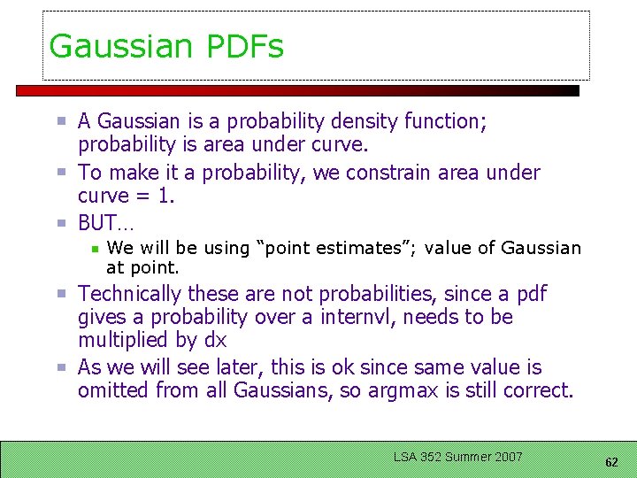
Gaussian PDFs A Gaussian is a probability density function; probability is area under curve. To make it a probability, we constrain area under curve = 1. BUT… We will be using “point estimates”; value of Gaussian at point. Technically these are not probabilities, since a pdf gives a probability over a internvl, needs to be multiplied by dx As we will see later, this is ok since same value is omitted from all Gaussians, so argmax is still correct. LSA 352 Summer 2007 62

Gaussians for Acoustic Modeling A Gaussian is parameterized by a mean and a variance: Different means P(o|q): P(o|q) is highest here at mean P(o|q is low here, very far from mean) P(o|q) o LSA 352 Summer 2007 63

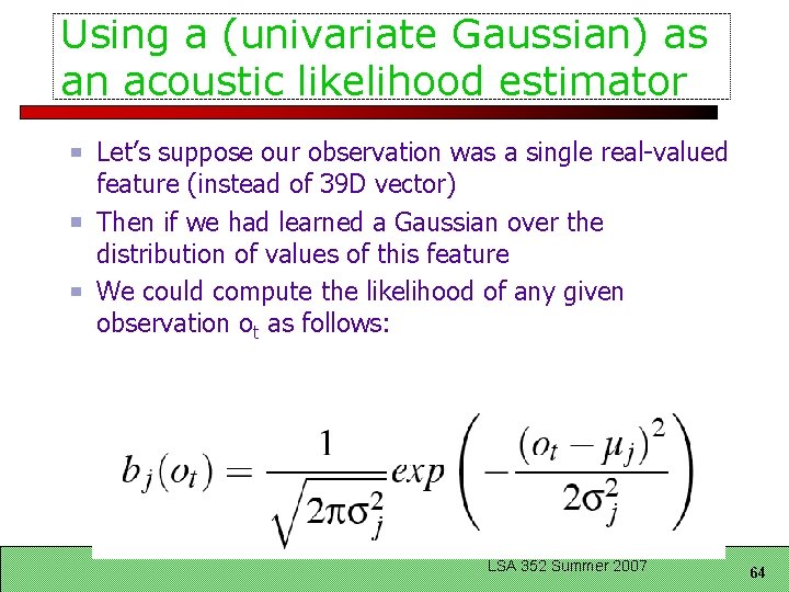
Using a (univariate Gaussian) as an acoustic likelihood estimator Let’s suppose our observation was a single real-valued feature (instead of 39 D vector) Then if we had learned a Gaussian over the distribution of values of this feature We could compute the likelihood of any given observation ot as follows: LSA 352 Summer 2007 64

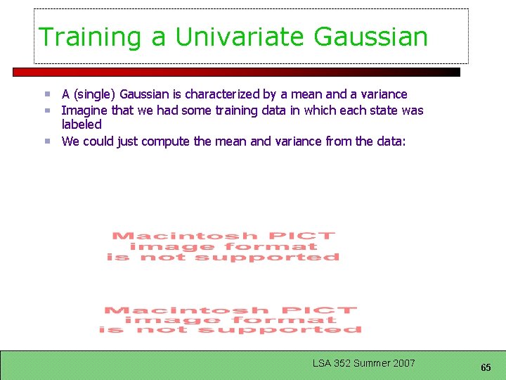
Training a Univariate Gaussian A (single) Gaussian is characterized by a mean and a variance Imagine that we had some training data in which each state was labeled We could just compute the mean and variance from the data: LSA 352 Summer 2007 65

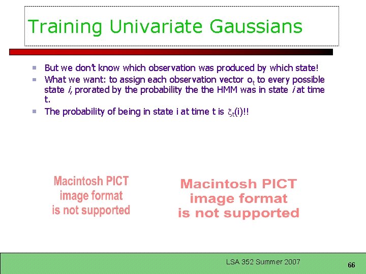
Training Univariate Gaussians But we don’t know which observation was produced by which state! What we want: to assign each observation vector ot to every possible state i, prorated by the probability the HMM was in state i at time t. The probability of being in state i at time t is t(i)!! LSA 352 Summer 2007 66

Multivariate Gaussians Instead of a single mean and variance : Vector of means and covariance matrix LSA 352 Summer 2007 67

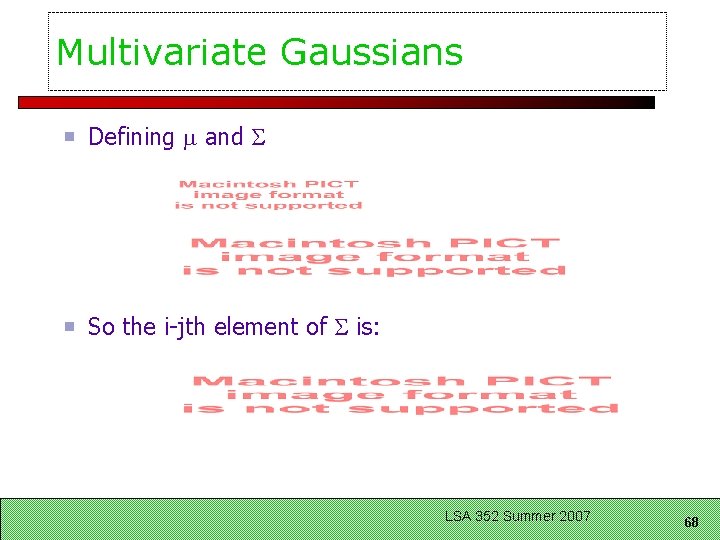
Multivariate Gaussians Defining and So the i-jth element of is: LSA 352 Summer 2007 68

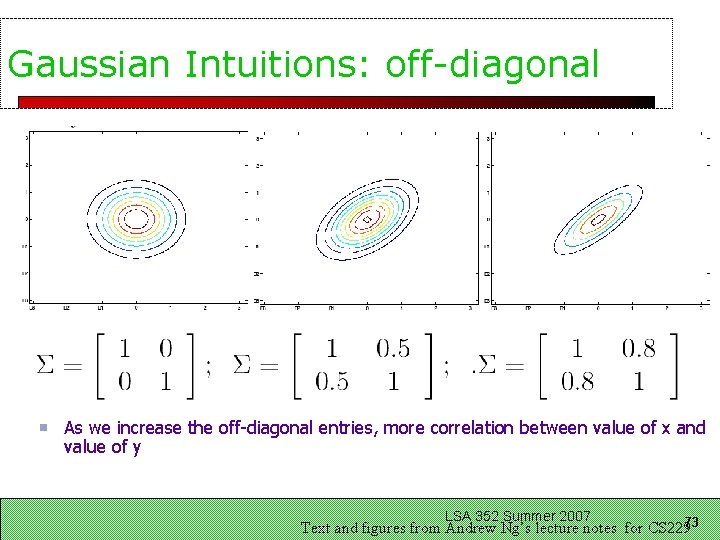
Gaussian Intuitions: Size of = [0 0] =I = 0. 6 I = 2 I As becomes larger, Gaussian becomes more spread out; as becomes smaller, Gaussian more compressed LSA 352 Summer 2007 Text and figures from Andrew Ng’s lecture notes for CS 22969

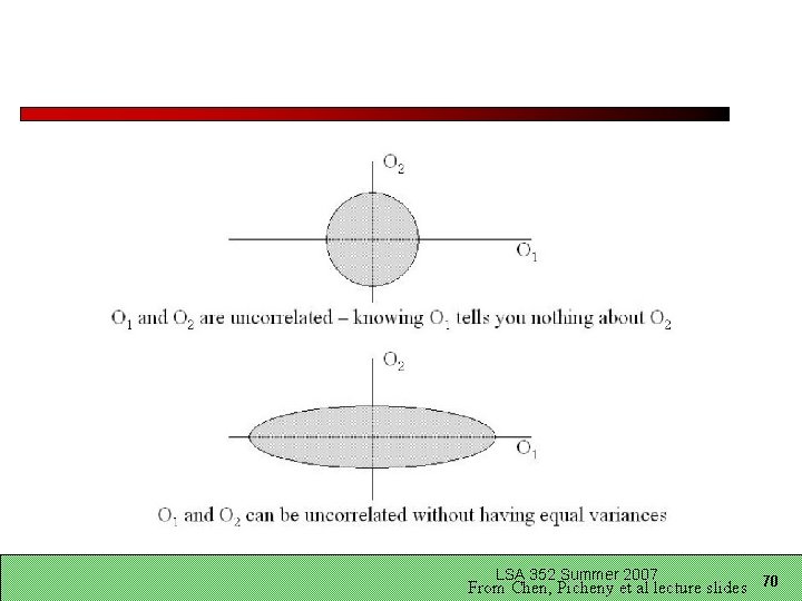
LSA 352 Summer 2007 From Chen, Picheny et al lecture slides 70

[1 0] [0 1] [. 6 0] [ 0 2] Different variances in different dimensions LSA 352 Summer 2007 71

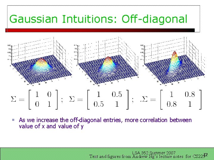
Gaussian Intuitions: Off-diagonal As we increase the off-diagonal entries, more correlation between value of x and value of y LSA 352 Summer 2007 Text and figures from Andrew Ng’s lecture notes for CS 22972

Gaussian Intuitions: off-diagonal As we increase the off-diagonal entries, more correlation between value of x and value of y LSA 352 Summer 2007 Text and figures from Andrew Ng’s lecture notes for CS 22973

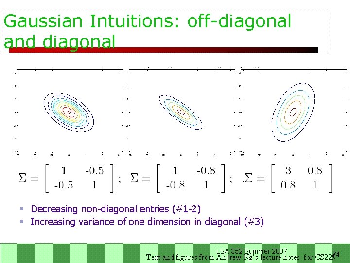
Gaussian Intuitions: off-diagonal and diagonal Decreasing non-diagonal entries (#1 -2) Increasing variance of one dimension in diagonal (#3) LSA 352 Summer 2007 Text and figures from Andrew Ng’s lecture notes for CS 22974

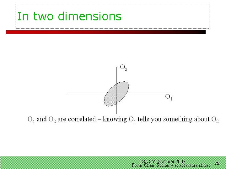
In two dimensions LSA 352 Summer 2007 From Chen, Picheny et al lecture slides 75

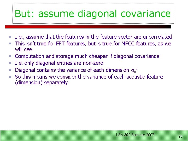
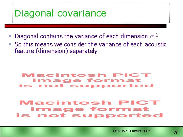
But: assume diagonal covariance I. e. , assume that the features in the feature vector are uncorrelated This isn’t true for FFT features, but is true for MFCC features, as we will see. Computation and storage much cheaper if diagonal covariance. I. e. only diagonal entries are non-zero Diagonal contains the variance of each dimension ii 2 So this means we consider the variance of each acoustic feature (dimension) separately LSA 352 Summer 2007 76

Diagonal covariance Diagonal contains the variance of each dimension ii 2 So this means we consider the variance of each acoustic feature (dimension) separately LSA 352 Summer 2007 77

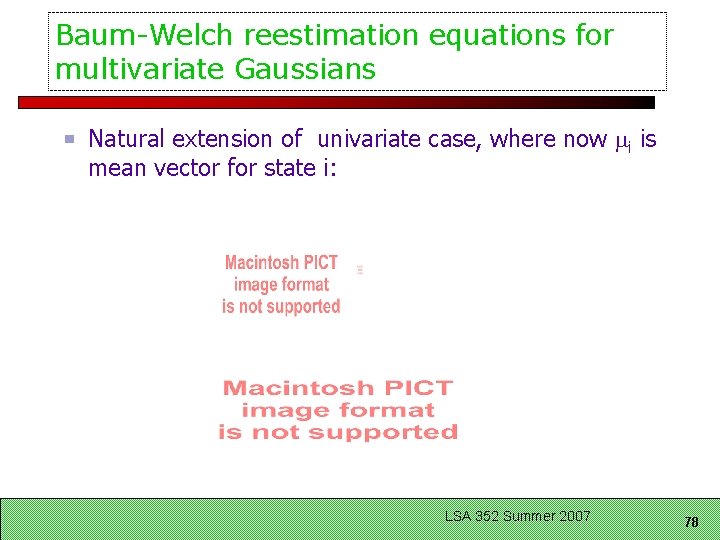
Baum-Welch reestimation equations for multivariate Gaussians Natural extension of univariate case, where now i is mean vector for state i: LSA 352 Summer 2007 78

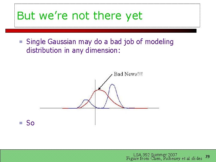
But we’re not there yet Single Gaussian may do a bad job of modeling distribution in any dimension: Solution: Mixtures of Gaussians LSA 352 Summer 2007 Figure from Chen, Picheney et al slides 79

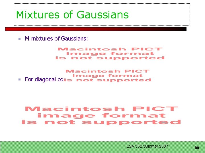
Mixtures of Gaussians M mixtures of Gaussians: For diagonal covariance: LSA 352 Summer 2007 80

GMMs Summary: each state has a likelihood function parameterized by: M Mixture weights M Mean Vectors of dimensionality D Either – M Covariance Matrices of Dx. D Or more likely – M Diagonal Covariance Matrices of Dx. D – which is equivalent to – M Variance Vectors of dimensionality D LSA 352 Summer 2007 81

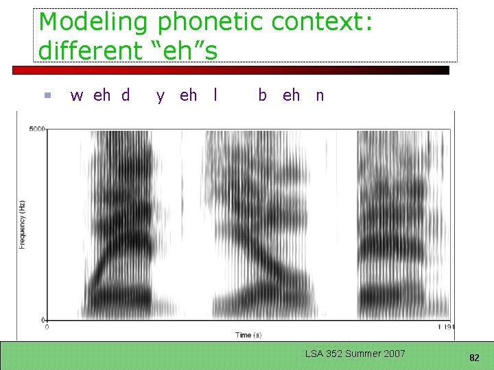
Modeling phonetic context: different “eh”s w eh d y eh l b eh n LSA 352 Summer 2007 82

Modeling phonetic context The strongest factor affecting phonetic variability is the neighboring phone How to model that in HMMs? Idea: have phone models which are specific to context. Instead of Context-Independent (CI) phones We’ll have Context-Dependent (CD) phones LSA 352 Summer 2007 83

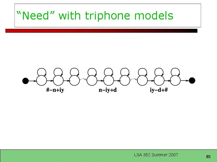
CD phones: triphones Triphones Each triphone captures facts about preceding and following phone Monophone: p, t, k Triphone: iy-p+aa a-b+c means “phone b, preceding by phone a, followed by phone c” LSA 352 Summer 2007 84

“Need” with triphone models LSA 352 Summer 2007 85

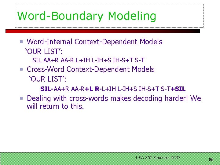
Word-Boundary Modeling Word-Internal Context-Dependent Models ‘OUR LIST’: SIL AA+R AA-R L+IH L-IH+S IH-S+T S-T Cross-Word Context-Dependent Models ‘OUR LIST’: SIL-AA+R AA-R+L R-L+IH L-IH+S IH-S+T S-T+SIL Dealing with cross-words makes decoding harder! We will return to this. LSA 352 Summer 2007 86

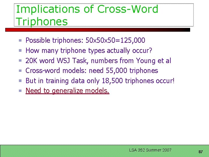
Implications of Cross-Word Triphones Possible triphones: 50 x 50=125, 000 How many triphone types actually occur? 20 K word WSJ Task, numbers from Young et al Cross-word models: need 55, 000 triphones But in training data only 18, 500 triphones occur! Need to generalize models. LSA 352 Summer 2007 87

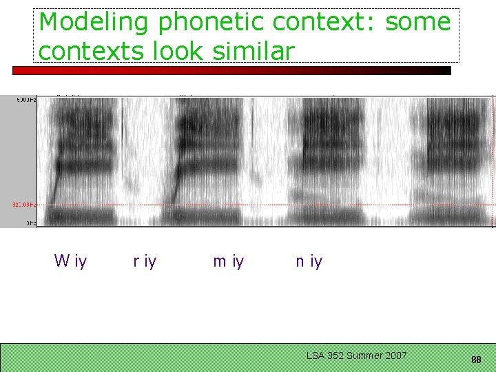
Modeling phonetic context: some contexts look similar W iy r iy m iy n iy LSA 352 Summer 2007 88

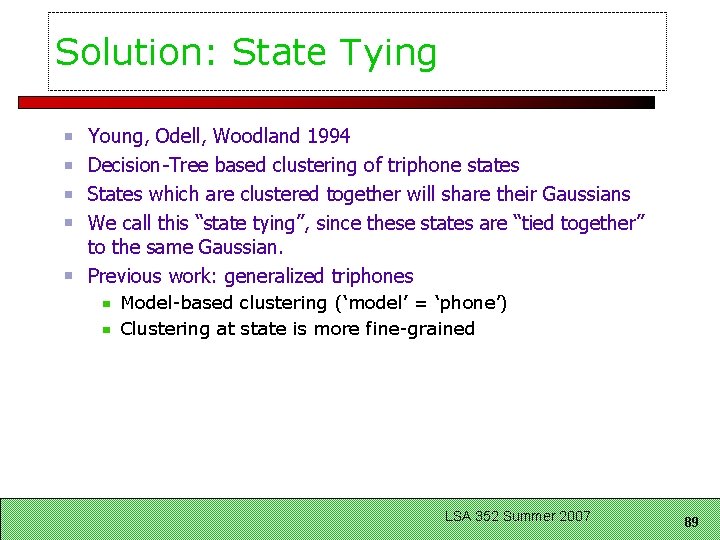
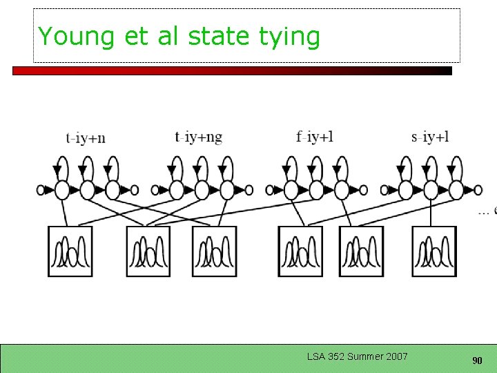
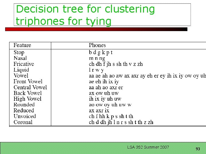
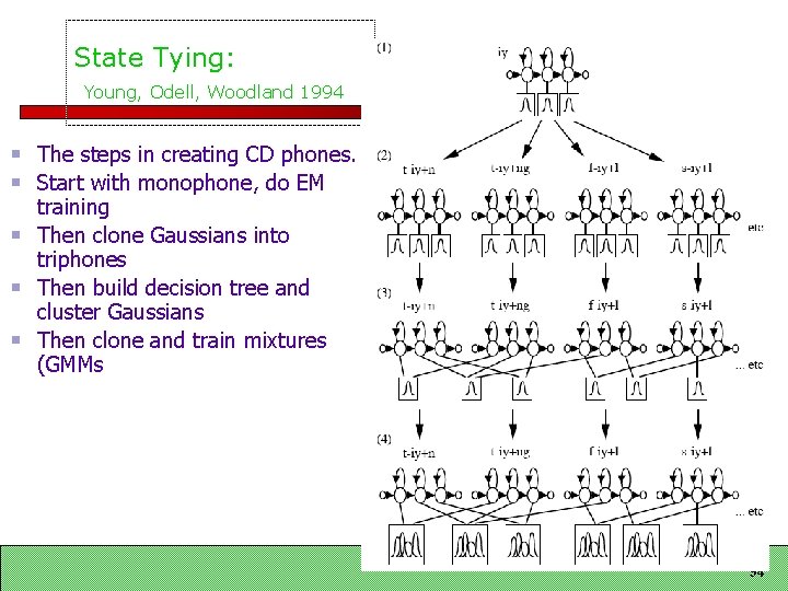
Solution: State Tying Young, Odell, Woodland 1994 Decision-Tree based clustering of triphone states States which are clustered together will share their Gaussians We call this “state tying”, since these states are “tied together” to the same Gaussian. Previous work: generalized triphones Model-based clustering (‘model’ = ‘phone’) Clustering at state is more fine-grained LSA 352 Summer 2007 89

Young et al state tying LSA 352 Summer 2007 90

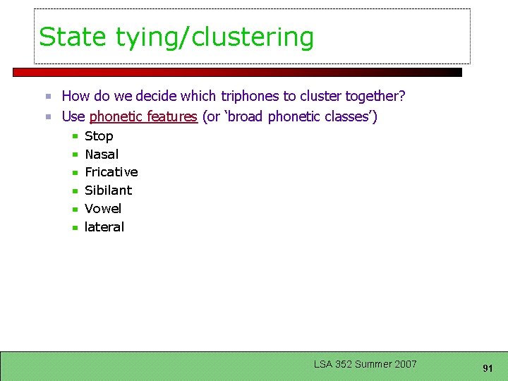
State tying/clustering How do we decide which triphones to cluster together? Use phonetic features (or ‘broad phonetic classes’) Stop Nasal Fricative Sibilant Vowel lateral LSA 352 Summer 2007 91

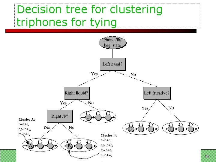
Decision tree for clustering triphones for tying LSA 352 Summer 2007 92

Decision tree for clustering triphones for tying LSA 352 Summer 2007 93

State Tying: Young, Odell, Woodland 1994 The steps in creating CD phones. Start with monophone, do EM training Then clone Gaussians into triphones Then build decision tree and cluster Gaussians Then clone and train mixtures (GMMs LSA 352 Summer 2007 94

Evaluation How to evaluate the word string output by a speech recognizer? LSA 352 Summer 2007 95

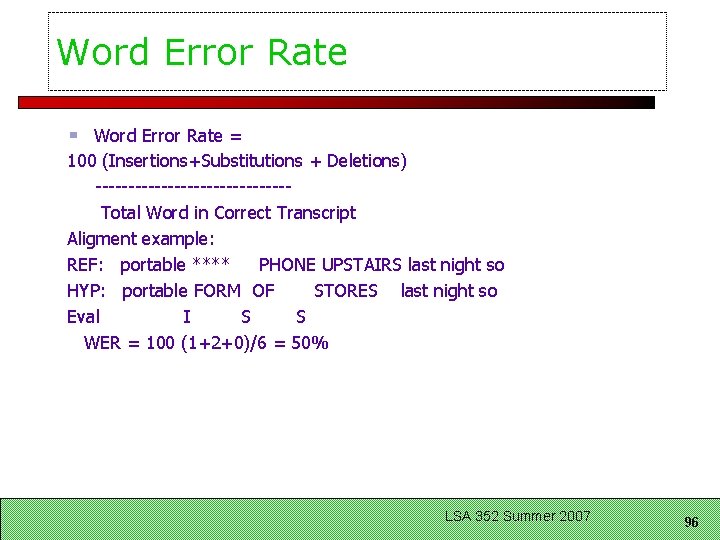
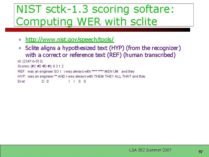
Word Error Rate = 100 (Insertions+Substitutions + Deletions) ---------------Total Word in Correct Transcript Aligment example: REF: portable **** PHONE UPSTAIRS last night so HYP: portable FORM OF STORES last night so Eval I S S WER = 100 (1+2+0)/6 = 50% LSA 352 Summer 2007 96

NIST sctk-1. 3 scoring softare: Computing WER with sclite http: //www. nist. gov/speech/tools/ Sclite aligns a hypothesized text (HYP) (from the recognizer) with a correct or reference text (REF) (human transcribed) id: (2347 -b-013) Scores: (#C #S #D #I) 9 3 1 2 REF: was an engineer SO I i was always with **** MEN UM and they HYP: was an engineer ** AND i was always with THEM THEY ALL THAT and they Eval: D S I I S S LSA 352 Summer 2007 97

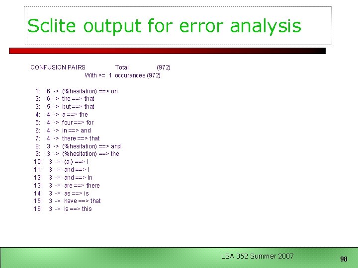
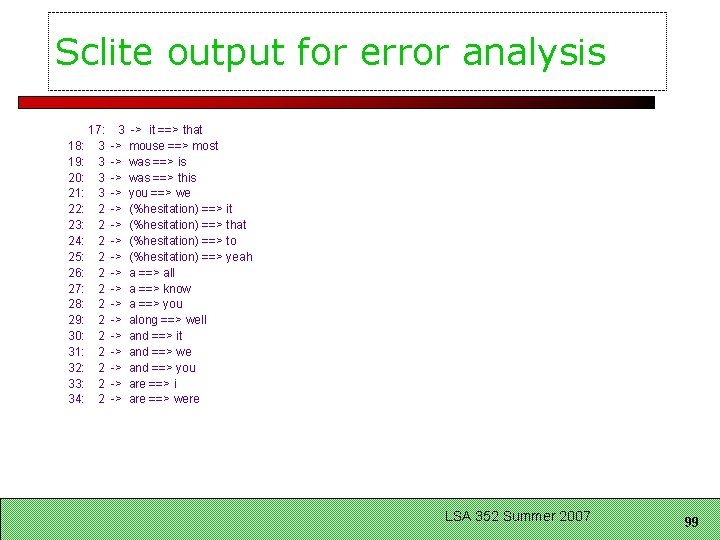
Sclite output for error analysis CONFUSION PAIRS Total (972) With >= 1 occurances (972) 1: 2: 3: 4: 5: 6: 7: 8: 9: 10: 11: 12: 13: 14: 15: 16: 6 -> (%hesitation) ==> on 6 -> the ==> that 5 -> but ==> that 4 -> a ==> the 4 -> four ==> for 4 -> in ==> and 4 -> there ==> that 3 -> (%hesitation) ==> and 3 -> (%hesitation) ==> the 3 -> (a-) ==> i 3 -> and ==> in 3 -> are ==> there 3 -> as ==> is 3 -> have ==> that 3 -> is ==> this LSA 352 Summer 2007 98

Sclite output for error analysis 18: 19: 20: 21: 22: 23: 24: 25: 26: 27: 28: 29: 30: 31: 32: 33: 34: 17: 3 3 2 2 2 2 3 -> -> -> -> -> it ==> that mouse ==> most was ==> is was ==> this you ==> we (%hesitation) ==> it (%hesitation) ==> that (%hesitation) ==> to (%hesitation) ==> yeah a ==> all a ==> know a ==> you along ==> well and ==> it and ==> we and ==> you are ==> i are ==> were LSA 352 Summer 2007 99

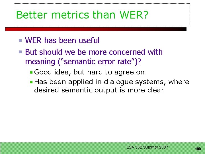
Better metrics than WER? WER has been useful But should we be more concerned with meaning (“semantic error rate”)? Good idea, but hard to agree on Has been applied in dialogue systems, where desired semantic output is more clear LSA 352 Summer 2007 100

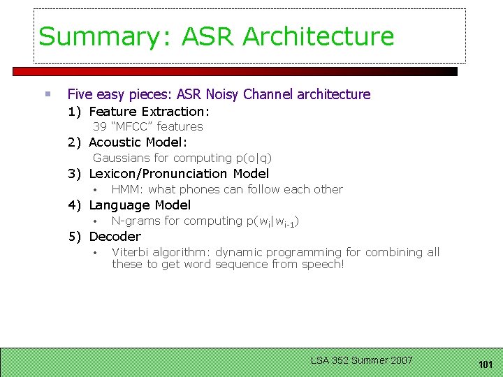
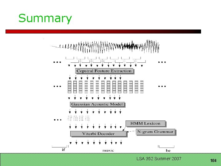
Summary: ASR Architecture Five easy pieces: ASR Noisy Channel architecture 1) Feature Extraction: 39 “MFCC” features 2) Acoustic Model: Gaussians for computing p(o|q) 3) Lexicon/Pronunciation Model • HMM: what phones can follow each other 4) Language Model • N-grams for computing p(wi|wi-1) 5) Decoder • Viterbi algorithm: dynamic programming for combining all these to get word sequence from speech! LSA 352 Summer 2007 101

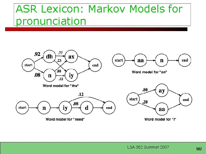
ASR Lexicon: Markov Models for pronunciation LSA 352 Summer 2007 102

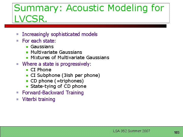
Summary: Acoustic Modeling for LVCSR. Increasingly sophisticated models For each state: Gaussians Multivariate Gaussians Mixtures of Multivariate Gaussians Where a state is progressively: CI Phone CI Subphone (3 ish per phone) CD phone (=triphones) State-tying of CD phone Forward-Backward Training Viterbi training LSA 352 Summer 2007 103

Summary LSA 352 Summer 2007 104