LQR Linear Quadratic Regulator A state space optimal

LQR Linear Quadratic Regulator A state space optimal control technique Brett Shapiro G 1400100 -v 1 1

Summary • LQR description • LQR derivation – Double pendulum test mass control example • LQR observer formulation – Quad pendulum damping observer example • Augmenting the plant for more complexity – Example: Frequency domain LQR 2

References • Reference 1: Modern Control Engineering, 4 th Ed. Katsuhiko Ogata. 2002, Prentice Hall. • Reference 2: Linear Optimal Control Systems. Huibert Kwakernaak, Raphael Sivan. 1972, Wiley. Interscience. Online access at http: //www. ieeecss. org/publications/classicbooks • Reference 3: T 1300301 – LQR in the frequency domain 3

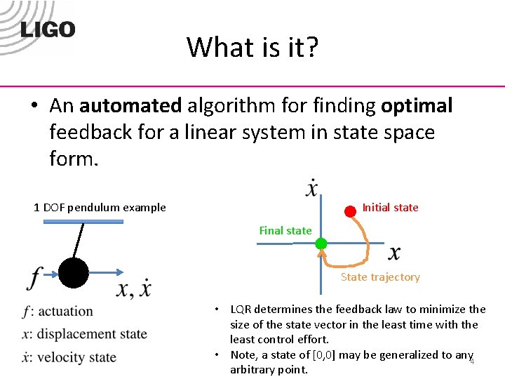
What is it? • An automated algorithm for finding optimal feedback for a linear system in state space form. 1 DOF pendulum example Initial state Final state State trajectory • LQR determines the feedback law to minimize the size of the state vector in the least time with the least control effort. • Note, a state of [0, 0] may be generalized to any 4 arbitrary point.

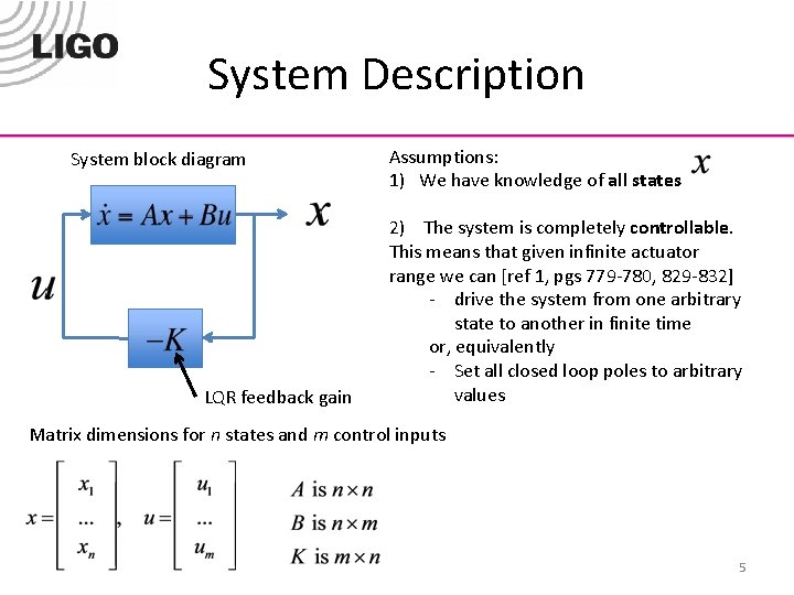
System Description System block diagram LQR feedback gain Assumptions: 1) We have knowledge of all states 2) The system is completely controllable. This means that given infinite actuator range we can [ref 1, pgs 779 -780, 829 -832] - drive the system from one arbitrary state to another in finite time or, equivalently - Set all closed loop poles to arbitrary values Matrix dimensions for n states and m control inputs 5

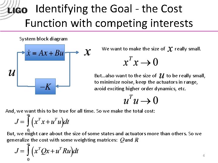
Identifying the Goal - the Cost Function with competing interests System block diagram We want to make the size of really small. But…also want to the size of to be really small, to minimize noise, keep the actuators in range, avoid exciting higher order dynamics, etc. And, we want this to be true for all time. So we make the total cost: But, we might care about the size of some states and actuators more than others. So we generalize the cost with some weighting matrices: and 6

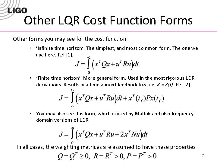
Other LQR Cost Function Forms Other forms you may see for the cost function • ‘Infinite time horizon’. The simplest, and most common form. The one we use here. Ref [1]. • ‘Finite time horizon’. More general form. Used in the most rigorous LQR derivations. Results in a time variant feedback law, i. e. K = K(t). Ref [2]. • You may also see this form, which is used by Matlab and also frequency domain versions of LQR. In all cases, the weighting matrices are assumed to have these properties 7

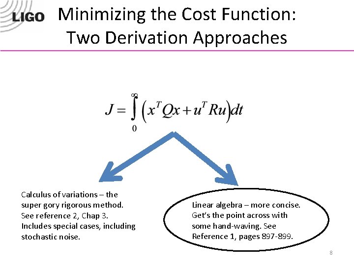
Minimizing the Cost Function: Two Derivation Approaches Calculus of variations – the super gory rigorous method. See reference 2, Chap 3. Includes special cases, including stochastic noise. Linear algebra – more concise. Get’s the point across with some hand-waving. See Reference 1, pages 897 -899. 8

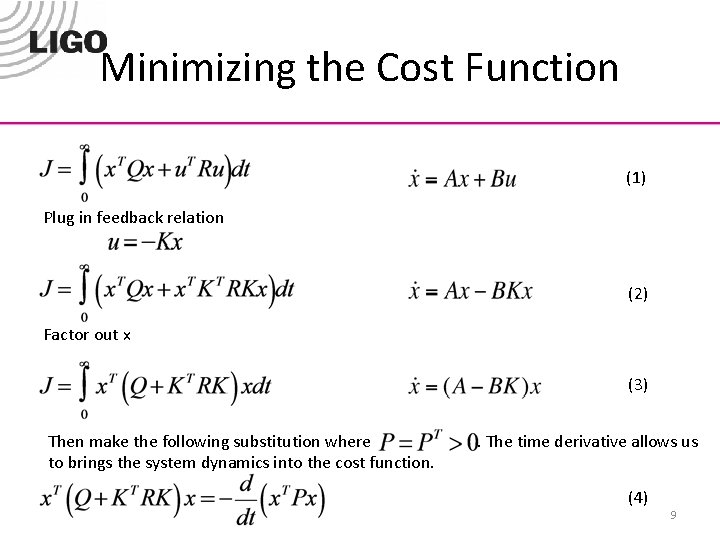
Minimizing the Cost Function (1) Plug in feedback relation (2) Factor out x (3) Then make the following substitution where to brings the system dynamics into the cost function. . The time derivative allows us (4) 9

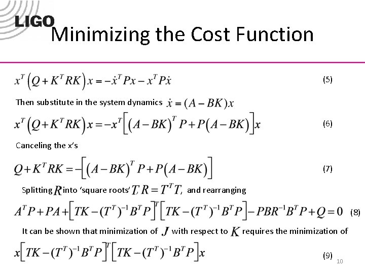
Minimizing the Cost Function (5) Then substitute in the system dynamics (6) Canceling the x’s (7) Splitting into ‘square roots’ , , and rearranging (8) It can be shown that minimization of with respect to requires the minimization of (9) 10

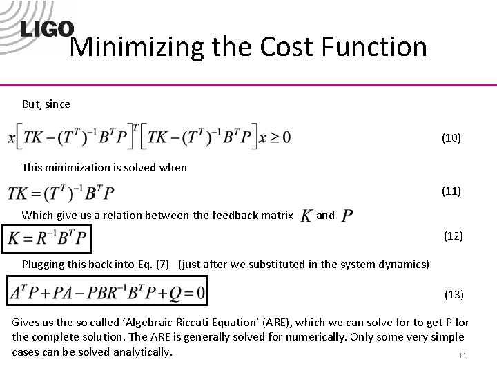
Minimizing the Cost Function But, since (10) This minimization is solved when (11) Which give us a relation between the feedback matrix and (12) Plugging this back into Eq. (7) (just after we substituted in the system dynamics) (13) Gives us the so called ‘Algebraic Riccati Equation’ (ARE), which we can solve for to get P for the complete solution. The ARE is generally solved for numerically. Only some very simple cases can be solved analytically. 11

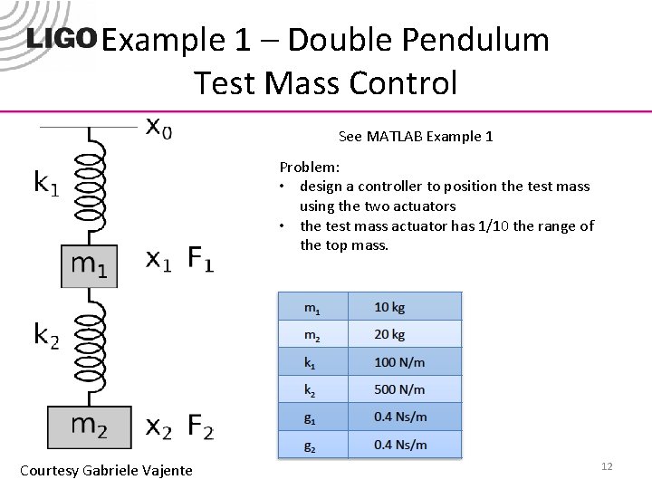
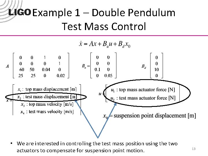
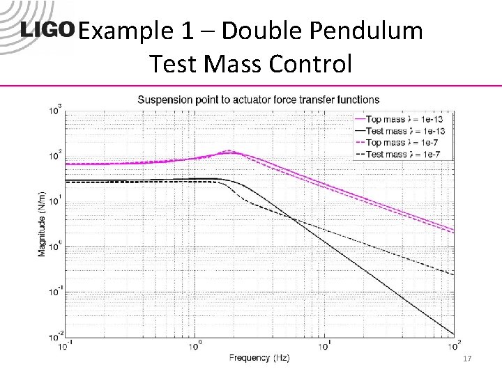
Example 1 – Double Pendulum Test Mass Control See MATLAB Example 1 Problem: • design a controller to position the test mass using the two actuators • the test mass actuator has 1/10 the range of the top mass. Courtesy Gabriele Vajente 12

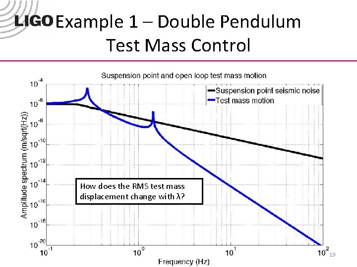
Example 1 – Double Pendulum Test Mass Control • We are interested in controlling the test mass position using the two actuators to compensate for suspension point motion. 13

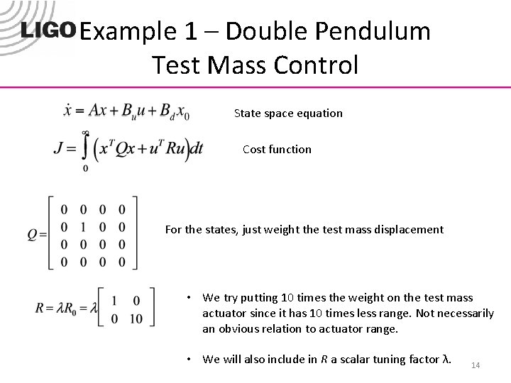
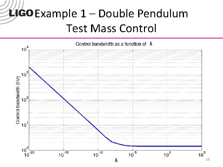
Example 1 – Double Pendulum Test Mass Control State space equation Cost function For the states, just weight the test mass displacement • We try putting 10 times the weight on the test mass actuator since it has 10 times less range. Not necessarily an obvious relation to actuator range. • We will also include in R a scalar tuning factor λ. 14

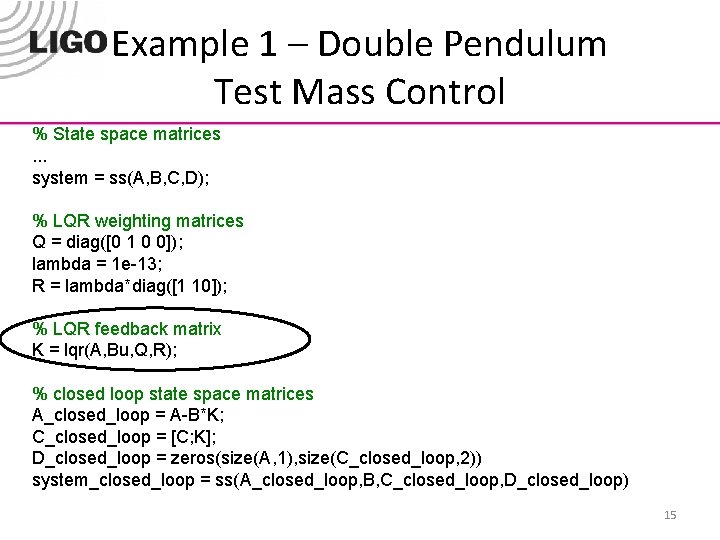
Example 1 – Double Pendulum Test Mass Control % State space matrices. . . system = ss(A, B, C, D); % LQR weighting matrices Q = diag([0 1 0 0]); lambda = 1 e-13; R = lambda*diag([1 10]); % LQR feedback matrix K = lqr(A, Bu, Q, R); % closed loop state space matrices A_closed_loop = A-B*K; C_closed_loop = [C; K]; D_closed_loop = zeros(size(A, 1), size(C_closed_loop, 2)) system_closed_loop = ss(A_closed_loop, B, C_closed_loop, D_closed_loop) 15

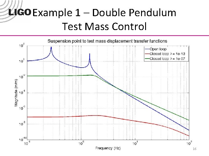
Example 1 – Double Pendulum Test Mass Control 16

Example 1 – Double Pendulum Test Mass Control 17

Example 1 – Double Pendulum Test Mass Control λ λ 18

Example 1 – Double Pendulum Test Mass Control How does the RMS test mass displacement change with λ? 19

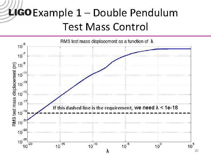
Example 1 – Double Pendulum Test Mass Control λ If this dashed line is the requirement, we need λ < 1 e-18 λ 20

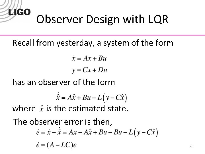
Observer Design with LQR Recall from yesterday, a system of the form has an observer of the form where is the estimated state. The observer error is then, 21

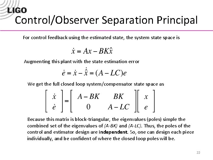
Control/Observer Separation Principal For control feedback using the estimated state, the system state space is Augmenting this plant with the state estimation error We get the full closed loop system/compensator state space as Because this matrix is block-triangular, the eigenvalues (poles) simple the combined set of the eigenvalues of (A-BK) and (A-LC). Thus, the poles of the control and estimator design are independent. So, one can design each piece individually, and be confident of where the closed loop poles will be. 22

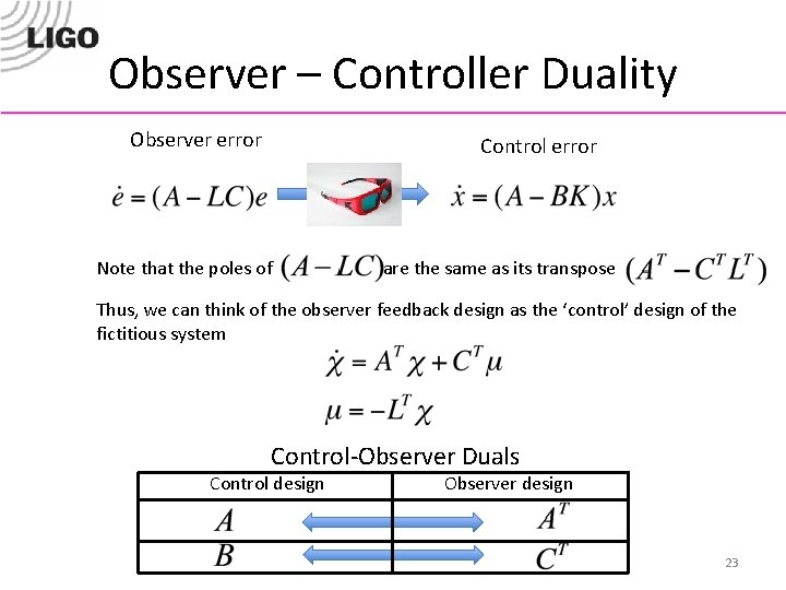
Observer – Controller Duality Observer error Control error Note that the poles of are the same as its transpose Thus, we can think of the observer feedback design as the ‘control’ design of the fictitious system Control-Observer Duals Control design Observer design 23

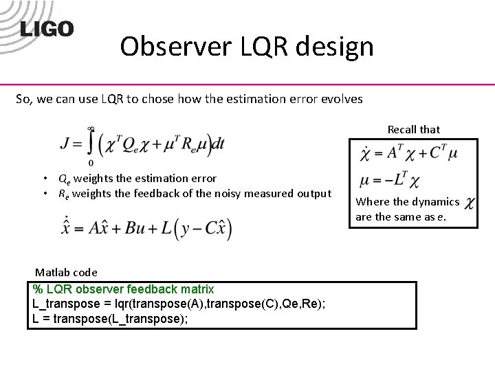
Observer LQR design So, we can use LQR to chose how the estimation error evolves Recall that • Qe weights the estimation error • Re weights the feedback of the noisy measured output Matlab code % LQR observer feedback matrix L_transpose = lqr(transpose(A), transpose(C), Qe, Re); L = transpose(L_transpose); Where the dynamics are the same as e.

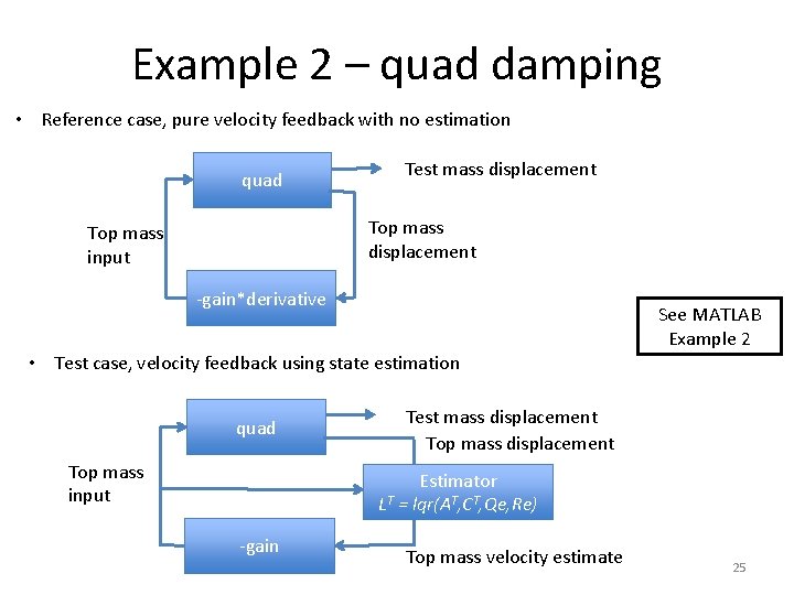
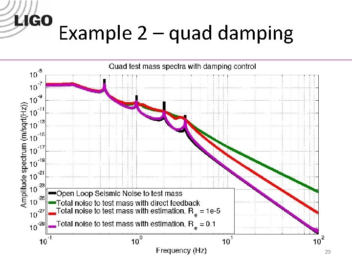
Example 2 – quad damping • Reference case, pure velocity feedback with no estimation quad Test mass displacement Top mass input -gain*derivative See MATLAB Example 2 • Test case, velocity feedback using state estimation quad Top mass input Test mass displacement Top mass displacement Estimator LT = lqr(AT, CT, Qe, Re) -gain Top mass velocity estimate 25

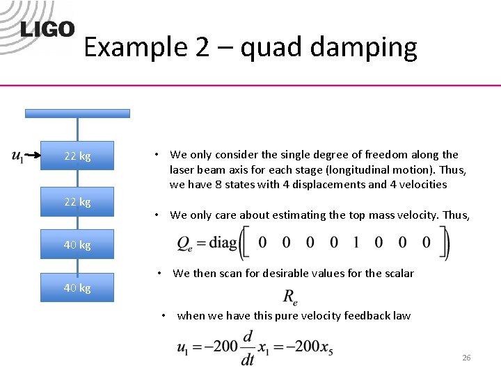
Example 2 – quad damping 22 kg • We only consider the single degree of freedom along the laser beam axis for each stage (longitudinal motion). Thus, we have 8 states with 4 displacements and 4 velocities • We only care about estimating the top mass velocity. Thus, 40 kg • We then scan for desirable values for the scalar • when we have this pure velocity feedback law 26

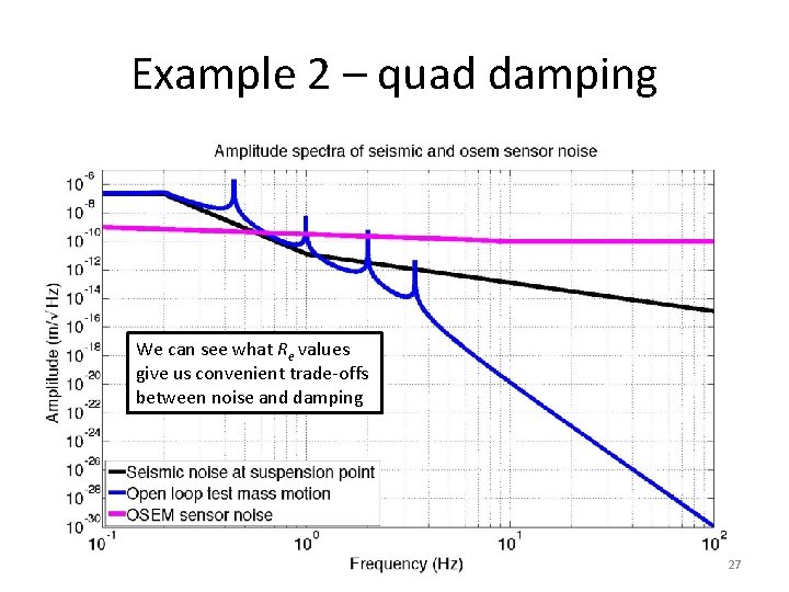
Example 2 – quad damping We can see what Re values give us convenient trade-offs between noise and damping 27

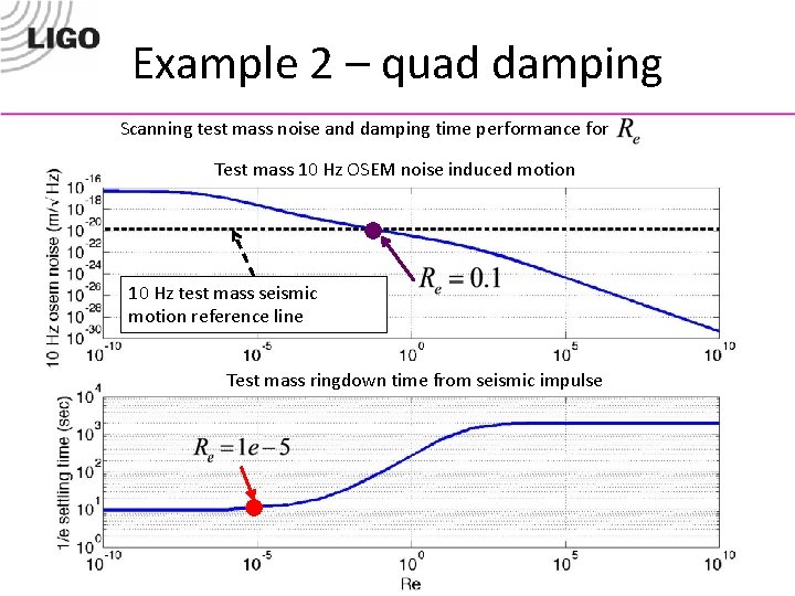
Example 2 – quad damping Scanning test mass noise and damping time performance for Test mass 10 Hz OSEM noise induced motion 10 Hz test mass seismic motion reference line Test mass ringdown time from seismic impulse 28

Example 2 – quad damping 29

Adding complexity – plant augmentation • One of LQR’s limitations is that the controller has no more complexity than the plant. Consequently, the controller design has finite degrees of freedom. • If we augment the plant with some fictitious states, we can achieve some more design degrees of freedom. 30

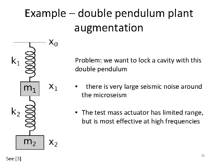
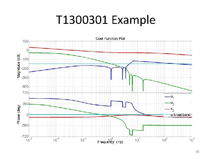
Example – double pendulum plant augmentation Problem: we want to lock a cavity with this double pendulum • there is very large seismic noise around the microseism • The test mass actuator has limited range, but is most effective at high frequencies See [3] 31

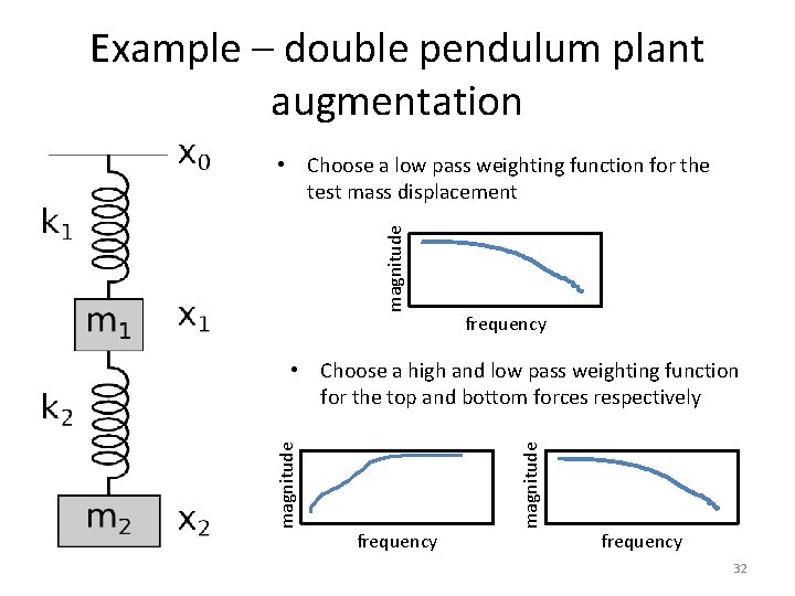
Example – double pendulum plant augmentation magnitude • Choose a low pass weighting function for the test mass displacement frequency magnitude • Choose a high and low pass weighting function for the top and bottom forces respectively frequency 32

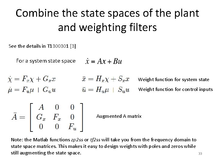
Combine the state spaces of the plant and weighting filters See the details in T 1300301 [3] For a system state space Weight function for system state Weight function for control inputs Augmented A matrix Note: the Matlab functions zp 2 ss or tf 2 ss will take you from the frequency domain to state space matrices. This makes it easy to design weights with poles and zeros while still augmenting the state space. 33

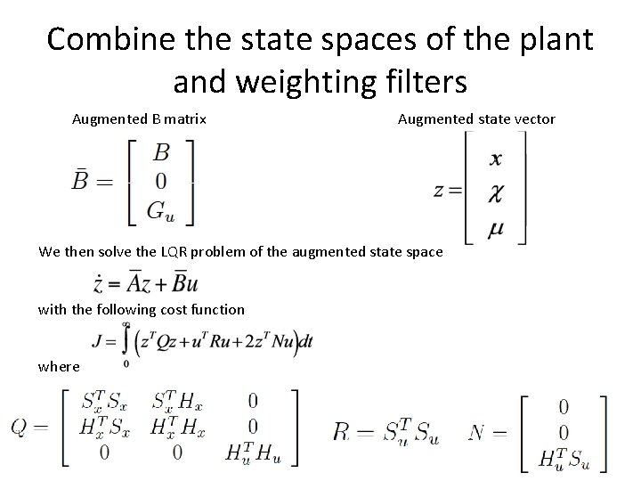
Combine the state spaces of the plant and weighting filters Augmented B matrix Augmented state vector We then solve the LQR problem of the augmented state space with the following cost function where

T 1300301 Example 35

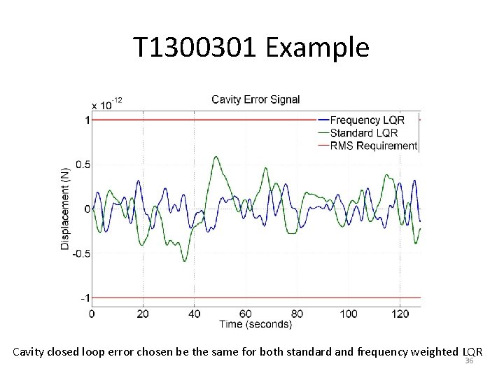
T 1300301 Example Cavity closed loop error chosen be the same for both standard and frequency weighted LQR 36

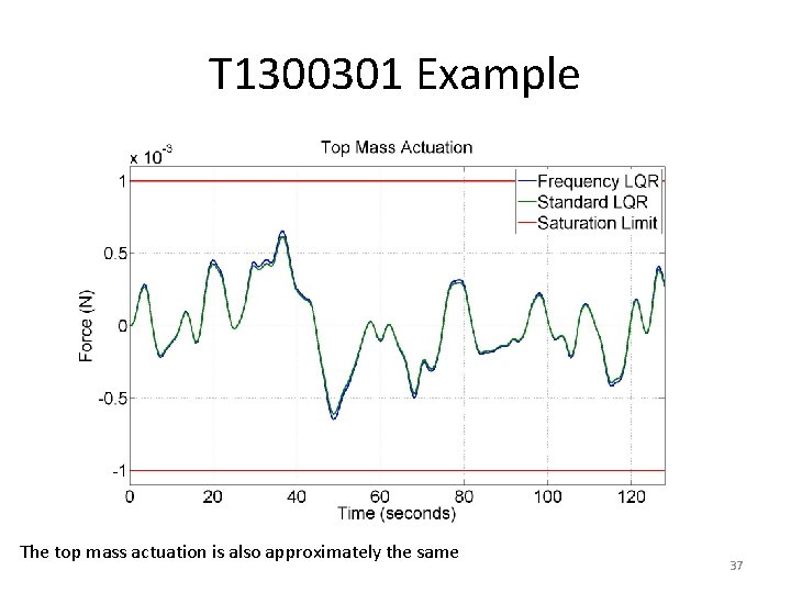
T 1300301 Example The top mass actuation is also approximately the same 37

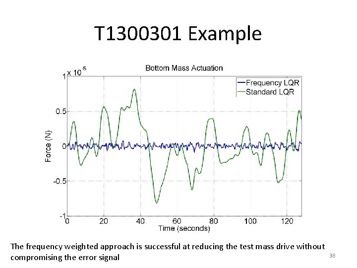
T 1300301 Example The frequency weighted approach is successful at reducing the test mass drive without compromising the error signal 38

Conclusions • LQR Benefits – Optimal solution to control problem – Automated (and very fast) method to design – Always stable with a good model – The controllers are typically robust • LQR Limitations – Only has as much complexity as the plant o This can be overcome by augmenting the plant – Identifying the best weighting matrices is an art 39

Backups 40

Intro to Observers/Estimators • A state observer estimates the state of a system based on the system measurements. – Useful if not all states are known, and/or they are measured with noisy sensors – The measurements can involve states and/or inputs – The system must be observable – Observability (dual of controllable) means that the full state can be reconstructed from the outputs in finite time (recall, controllability is the ability to drive the system to any state in finite time) Ref 1, Chapter 12 -5. 41