LowPower Design of Digital VLSI Circuits Linear Programming

Low-Power Design of Digital VLSI Circuits Linear Programming – A Mathematical Optimization Technique Vishwani D. Agrawal James J. Danaher Professor Dept. of Electrical and Computer Engineering Auburn University, Auburn, AL 36849 vagrawal@eng. auburn. edu http: //www. eng. auburn. edu/~vagrawal Copyright Agrawal, 2011 Lectures 9 and 10, : Linear Programming 1

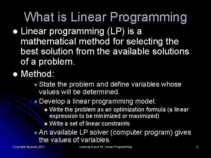
What is Linear Programming Linear programming (LP) is a mathematical method for selecting the best solution from the available solutions of a problem. l Method: l l State the problem and define variables whose values will be determined. l Develop a linear programming model: l l Write the problem as an optimization formula (a linear expression to be minimized or maximized) Write a set of linear constraints l An available LP solver (computer program) gives the values of variables. Copyright Agrawal, 2011 Lectures 9 and 10, : Linear Programming 2

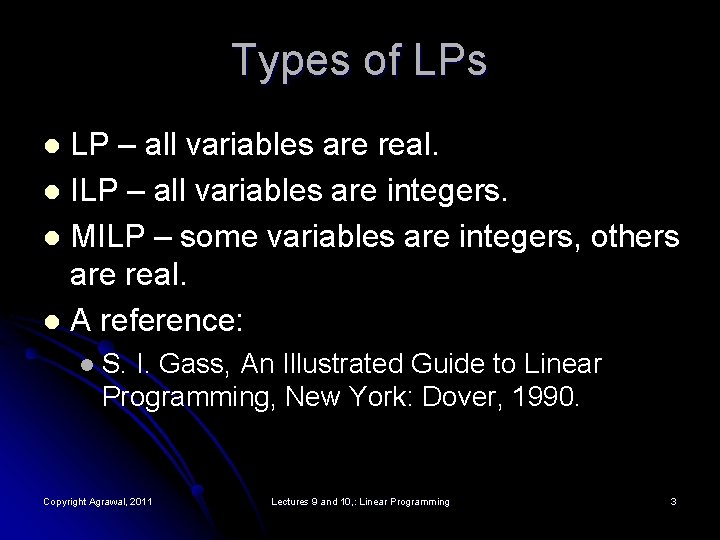
Types of LPs LP – all variables are real. l ILP – all variables are integers. l MILP – some variables are integers, others are real. l A reference: l l S. I. Gass, An Illustrated Guide to Linear Programming, New York: Dover, 1990. Copyright Agrawal, 2011 Lectures 9 and 10, : Linear Programming 3

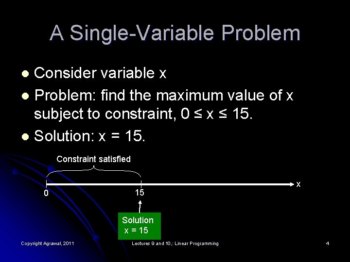
A Single-Variable Problem Consider variable x l Problem: find the maximum value of x subject to constraint, 0 ≤ x ≤ 15. l Solution: x = 15. l Constraint satisfied 0 15 x Solution x = 15 Copyright Agrawal, 2011 Lectures 9 and 10, : Linear Programming 4

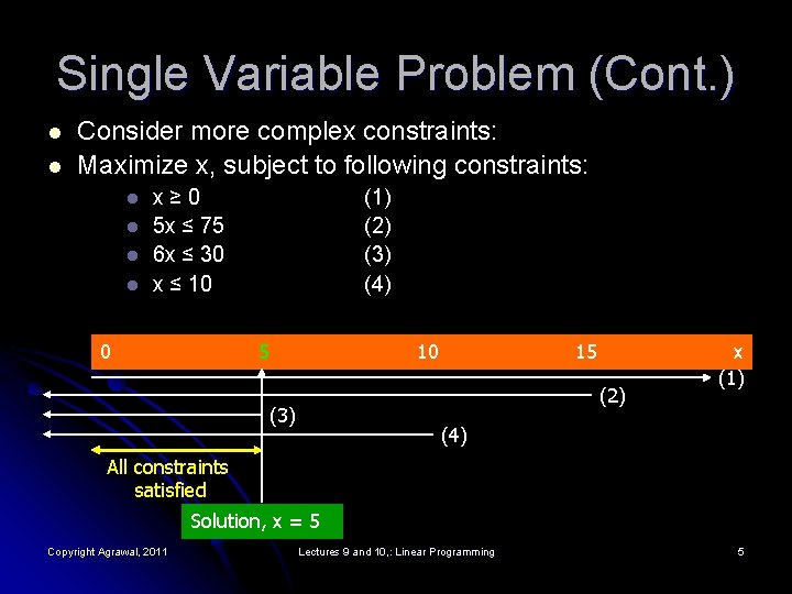
Single Variable Problem (Cont. ) l l Consider more complex constraints: Maximize x, subject to following constraints: l l x≥ 0 5 x ≤ 75 6 x ≤ 30 x ≤ 10 0 (1) (2) (3) (4) 5 10 15 (2) (3) x (1) (4) All constraints satisfied Solution, x = 5 Copyright Agrawal, 2011 Lectures 9 and 10, : Linear Programming 5

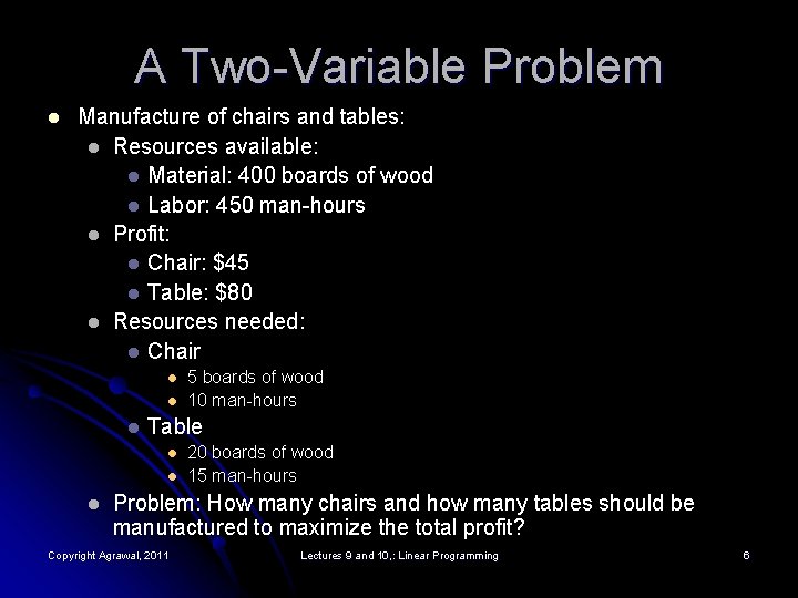
A Two-Variable Problem l Manufacture of chairs and tables: l Resources available: l Material: 400 boards of wood l Labor: 450 man-hours l Profit: l Chair: $45 l Table: $80 l Resources needed: l Chair l l l Table l l l 5 boards of wood 10 man-hours 20 boards of wood 15 man-hours Problem: How many chairs and how many tables should be manufactured to maximize the total profit? Copyright Agrawal, 2011 Lectures 9 and 10, : Linear Programming 6

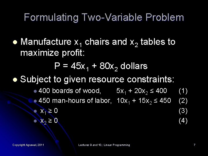
Formulating Two-Variable Problem Manufacture x 1 chairs and x 2 tables to maximize profit: P = 45 x 1 + 80 x 2 dollars l Subject to given resource constraints: l l 400 boards of wood, 5 x 1 + 20 x 2 ≤ 400 l 450 man-hours of labor, 10 x 1 + 15 x 2 ≤ 450 l x 1 ≥ 0 l x 2 ≥ 0 Copyright Agrawal, 2011 Lectures 9 and 10, : Linear Programming (1) (2) (3) (4) 7

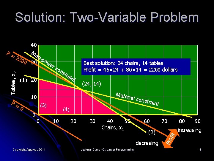
Solution: Two-Variable Problem n 00 30 -pow er co ns P= (1) 20 tra i Best solution: 24 chairs, 14 tables Profit = 45× 24 + 80× 14 = 2200 dollars nt (24, 14) Mater ia 10 l cons (3) 0 (4) 0 0 10 20 30 40 50 Chairs, x 1 traint 60 (2) decresing Copyright Agrawal, 2011 Lectures 9 and 10, : Linear Programming 70 80 90 increasing Pro fit 22 Tables, x 2 P= 40 Ma 8

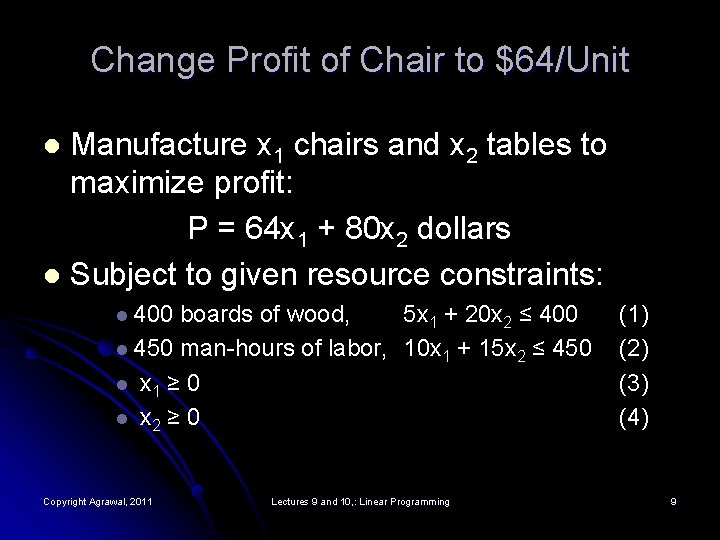
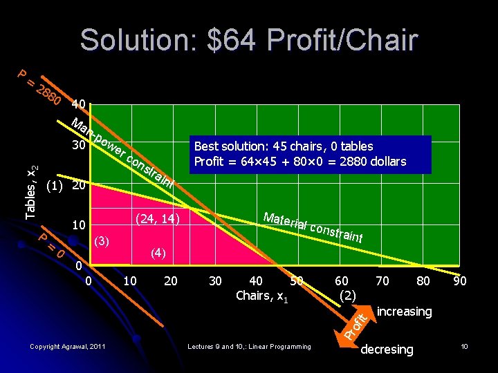
Change Profit of Chair to $64/Unit Manufacture x 1 chairs and x 2 tables to maximize profit: P = 64 x 1 + 80 x 2 dollars l Subject to given resource constraints: l l 400 boards of wood, 5 x 1 + 20 x 2 ≤ 400 l 450 man-hours of labor, 10 x 1 + 15 x 2 ≤ 450 l x 1 ≥ 0 l x 2 ≥ 0 Copyright Agrawal, 2011 Lectures 9 and 10, : Linear Programming (1) (2) (3) (4) 9

Solution: $64 Profit/Chair = 28 80 40 Ma n-p 30 owe rc Tables, x 2 P on s (1) 20 (3) 0 nt Mater ia (24, 14) 10 = tra i Best solution: 45 chairs, 0 tables Profit = 64× 45 + 80× 0 = 2880 dollars traint (4) 0 10 20 30 40 50 Chairs, x 1 60 (2) 70 it 0 l cons 80 90 increasing Pr of P Copyright Agrawal, 2011 Lectures 9 and 10, : Linear Programming decresing 10

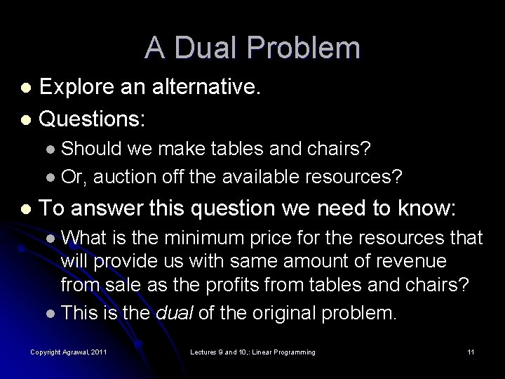
A Dual Problem Explore an alternative. l Questions: l Should we make tables and chairs? l Or, auction off the available resources? l l To answer this question we need to know: What is the minimum price for the resources that will provide us with same amount of revenue from sale as the profits from tables and chairs? l This is the dual of the original problem. l Copyright Agrawal, 2011 Lectures 9 and 10, : Linear Programming 11

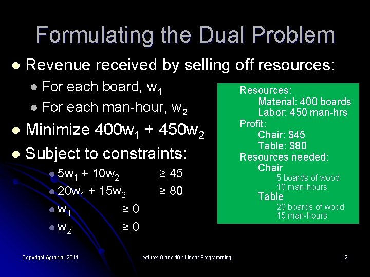
Formulating the Dual Problem l Revenue received by selling off resources: For each board, w 1 l For each man-hour, w 2 l Minimize 400 w 1 + 450 w 2 l Subject to constraints: l l 5 w 1 + 10 w 2 l 20 w 1 + 15 w 2 l w 1 ≥ 0 l w 2 ≥ 0 Copyright Agrawal, 2011 ≥ 45 ≥ 80 Lectures 9 and 10, : Linear Programming Resources: Material: 400 boards Labor: 450 man-hrs Profit: Chair: $45 Table: $80 Resources needed: Chair 5 boards of wood 10 man-hours Table 20 boards of wood 15 man-hours 12

The Duality Theorem l If the primal has a finite optimum solution, so does the dual, and the optimum values of the objective functions are equal. Copyright Agrawal, 2011 Lectures 9 and 10, : Linear Programming 13

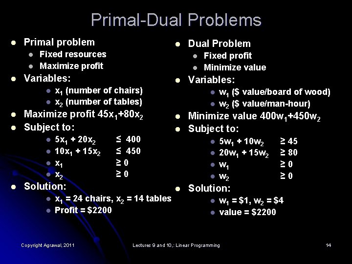
Primal-Dual Problems l Primal problem l l l Fixed resources Maximize profit l l l l x 1 (number of chairs) x 2 (number of tables) Maximize profit 45 x 1+80 x 2 Subject to: l 5 x 1 + 20 x 2 10 x 1 + 15 x 2 x 1 x 2 l Copyright Agrawal, 2011 Variables: l l l w 1 ($ value/board of wood) w 2 ($ value/man-hour) Minimize value 400 w 1+450 w 2 Subject to: l l l x 1 = 24 chairs, x 2 = 14 tables Profit = $2200 Fixed profit Minimize value l ≤ 400 ≤ 450 ≥ 0 Solution: l Dual Problem l Variables: l l l 5 w 1 + 10 w 2 20 w 1 + 15 w 2 w 1 w 2 ≥ 45 ≥ 80 ≥ 0 Solution: l l w 1 = $1, w 2 = $4 value = $2200 Lectures 9 and 10, : Linear Programming 14

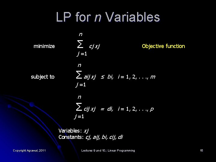
LP for n Variables n minimize Σ cj xj Objective function j =1 n subject to Σ aij xj ≤ bi, i = 1, 2, . . . , m j =1 n Σ cij xj = di, i = 1, 2, . . . , p j =1 Variables: xj Constants: cj, aij, bi, cij, di Copyright Agrawal, 2011 Lectures 9 and 10, : Linear Programming 15

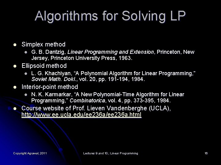
Algorithms for Solving LP l Simplex method l l Ellipsoid method l l L. G. Khachiyan, “A Polynomial Algorithm for Linear Programming, ” Soviet Math. Dokl. , vol. 20, pp. 191 -194, 1984. Interior-point method l l G. B. Dantzig, Linear Programming and Extension, Princeton, New Jersey, Princeton University Press, 1963. N. K. Karmarkar, “A New Polynomial-Time Algorithm for Linear Programming, ” Combinatorica, vol. 4, pp. 373 -395, 1984. Course website of Prof. Lieven Vandenberghe (UCLA), http: //www. ee. ucla. edu/ee 236 a. html Copyright Agrawal, 2011 Lectures 9 and 10, : Linear Programming 16

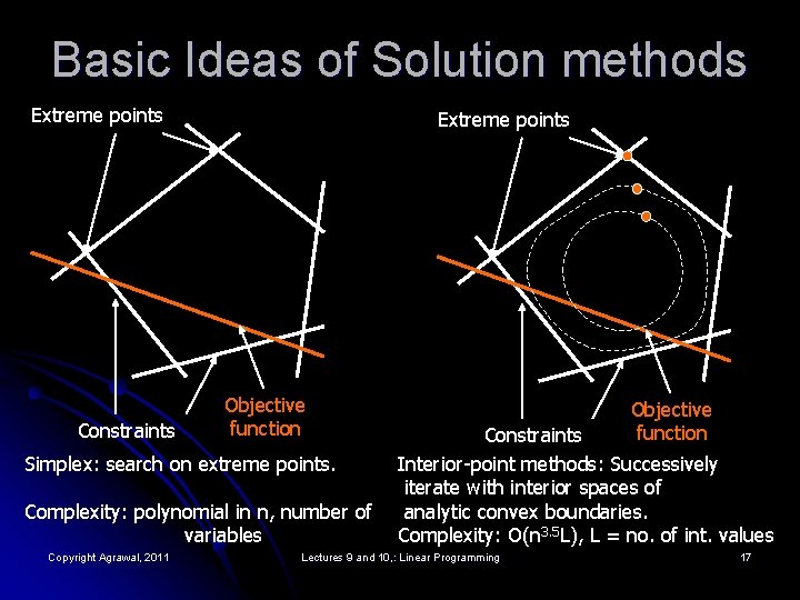
Basic Ideas of Solution methods Extreme points Constraints Extreme points Objective function Simplex: search on extreme points. Complexity: polynomial in n, number of variables Copyright Agrawal, 2011 Objective function Constraints Interior-point methods: Successively iterate with interior spaces of analytic convex boundaries. Complexity: O(n 3. 5 L), L = no. of int. values Lectures 9 and 10, : Linear Programming 17

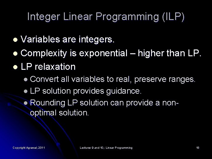
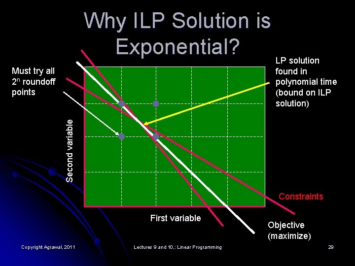
Integer Linear Programming (ILP) Variables are integers. l Complexity is exponential – higher than LP. l LP relaxation l l Convert all variables to real, preserve ranges. l LP solution provides guidance. l Rounding LP solution can provide a nonoptimal solution. Copyright Agrawal, 2011 Lectures 9 and 10, : Linear Programming 18

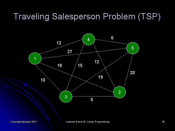
Traveling Salesperson Problem (TSP) 6 4 12 5 27 1 18 12 15 19 10 3 Copyright Agrawal, 2011 20 2 5 Lectures 9 and 10, : Linear Programming 19

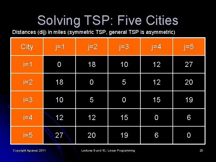
Solving TSP: Five Cities Distances (dij) in miles (symmetric TSP, general TSP is asymmetric) City j=1 j=2 j=3 j=4 j=5 i=1 0 18 10 12 27 i=2 18 0 5 12 20 i=3 10 5 0 15 19 i=4 12 12 15 0 6 i=5 27 20 19 6 0 Copyright Agrawal, 2011 Lectures 9 and 10, : Linear Programming 20

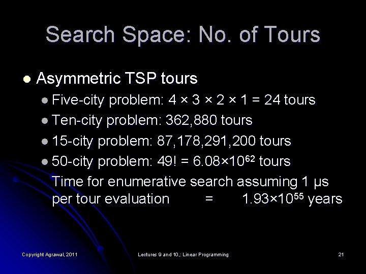
Search Space: No. of Tours l Asymmetric TSP tours l Five-city problem: 4 × 3 × 2 × 1 = 24 tours l Ten-city problem: 362, 880 tours l 15 -city problem: 87, 178, 291, 200 tours l 50 -city problem: 49! = 6. 08× 1062 tours Time for enumerative search assuming 1 μs per tour evaluation = 1. 93× 1055 years Copyright Agrawal, 2011 Lectures 9 and 10, : Linear Programming 21

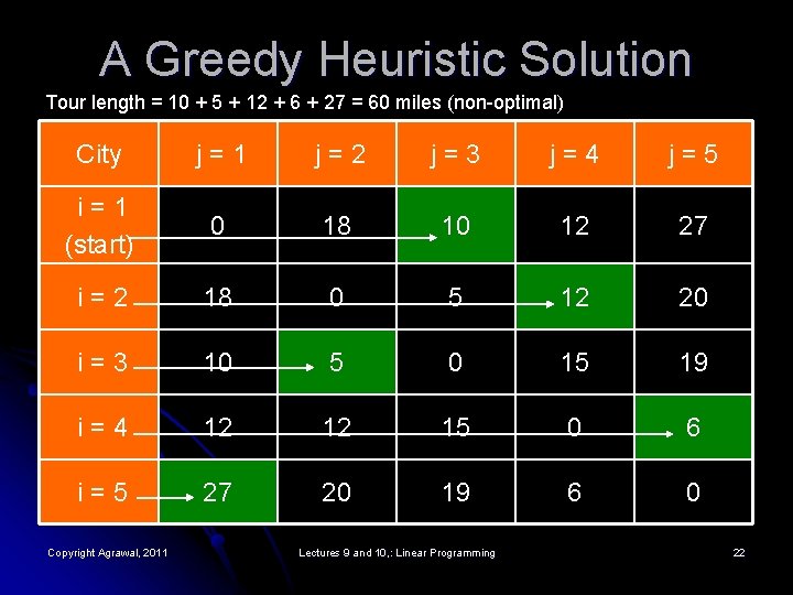
A Greedy Heuristic Solution Tour length = 10 + 5 + 12 + 6 + 27 = 60 miles (non-optimal) City j=1 j=2 j=3 j=4 j=5 i=1 (start) 0 18 10 12 27 i=2 18 0 5 12 20 i=3 10 5 0 15 19 i=4 12 12 15 0 6 i=5 27 20 19 6 0 Copyright Agrawal, 2011 Lectures 9 and 10, : Linear Programming 22

ILP Variables, Constants and Constraints x 14 ε [0, 1] d 14 = 12 4 5 x 15 ε [0, 1] d 15 = 27 x 12 ε [0, 1] d 12 = 18 1 x 13 ε [0, 1] d 13 = 10 Integer variables: xij = 1, travel i to j xij = 0, do not travel i to j 2 3 Real constants: dij = distance from i to j x 12 + x 13 + x 14 + x 15 = 1 four other similar equations Copyright Agrawal, 2011 Lectures 9 and 10, : Linear Programming 23

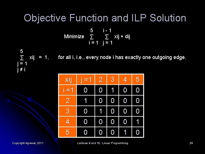
Objective Function and ILP Solution 5 i-1 Minimize ∑ ∑ xij × dij i=1 j=1 5 ∑ xij = 1, j=1 j≠i for all i, i. e. , every node i has exactly one outgoing edge. xij Copyright Agrawal, 2011 j =1 2 3 4 5 i =1 0 0 2 1 0 0 3 0 1 0 0 0 4 0 0 1 5 0 0 0 1 0 Lectures 9 and 10, : Linear Programming 24

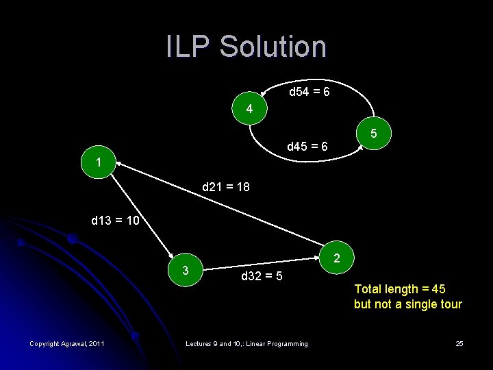
ILP Solution d 54 = 6 4 5 d 45 = 6 1 d 21 = 18 d 13 = 10 3 Copyright Agrawal, 2011 2 d 32 = 5 Lectures 9 and 10, : Linear Programming Total length = 45 but not a single tour 25

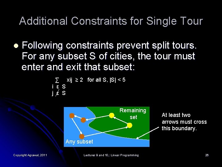
Additional Constraints for Single Tour l Following constraints prevent split tours. For any subset S of cities, the tour must enter and exit that subset: ∑ xij ≥ 2 for all S, |S| < 5 i ε S j ε S Remaining set At least two arrows must cross this boundary. Any subset Copyright Agrawal, 2011 Lectures 9 and 10, : Linear Programming 26

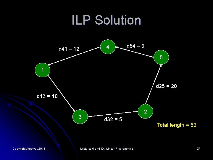
ILP Solution 4 d 41 = 12 d 54 = 6 5 1 d 25 = 20 d 13 = 10 3 Copyright Agrawal, 2011 2 d 32 = 5 Lectures 9 and 10, : Linear Programming Total length = 53 27

Characteristics of ILP l l l Worst-case complexity is exponential in number of variables. Linear programming (LP) relaxation, where integer variables are treated as real, gives a lower bound on the objective function. Recursive rounding of relaxed LP solution to nearest integers gives an approximate solution to the ILP problem. l K. R. Kantipudi and V. D. Agrawal, “A Reduced Complexity Algorithm for Minimizing N-Detect Tests, ” Proc. 20 th International Conf. VLSI Design, January 2007, pp. 492 -497. Copyright Agrawal, 2011 Lectures 9 and 10, : Linear Programming 28

Why ILP Solution is Exponential? LP solution Must try all 2 n roundoff points Second variable found in polynomial time (bound on ILP solution) Constraints First variable Copyright Agrawal, 2011 Lectures 9 and 10, : Linear Programming Objective (maximize) 29

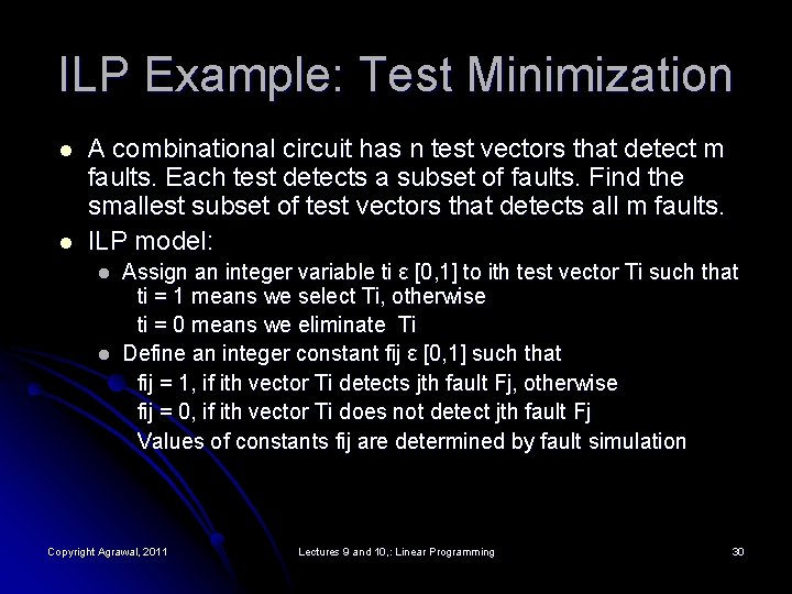
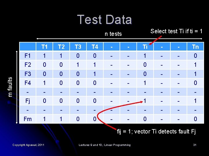
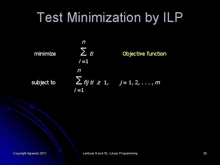
ILP Example: Test Minimization l l A combinational circuit has n test vectors that detect m faults. Each test detects a subset of faults. Find the smallest subset of test vectors that detects all m faults. ILP model: l l Assign an integer variable ti ε [0, 1] to ith test vector Ti such that ti = 1 means we select Ti, otherwise ti = 0 means we eliminate Ti Define an integer constant fij ε [0, 1] such that fij = 1, if ith vector Ti detects jth fault Fj, otherwise fij = 0, if ith vector Ti does not detect jth fault Fj Values of constants fij are determined by fault simulation Copyright Agrawal, 2011 Lectures 9 and 10, : Linear Programming 30

Test Data Select test Ti if ti = 1 m faults n tests T 1 T 2 T 3 T 4 - - Ti - - Tn F 1 1 1 0 0 - - 1 - - 0 F 2 0 0 1 1 - - 0 - - 1 F 3 0 0 0 1 - - 0 - - 1 F 4 1 0 0 0 - - 1 - - 0 - - - Fj 0 0 - - 1 - - - Fm 1 1 0 0 - - 0 fij = 1; vector Ti detects fault Fj Copyright Agrawal, 2011 Lectures 9 and 10, : Linear Programming 31

Test Minimization by ILP n minimize Σ ti Objective function i =1 n subject to Σ fij ti ≥ 1, j = 1, 2, . . . , m i =1 Copyright Agrawal, 2011 Lectures 9 and 10, : Linear Programming 32

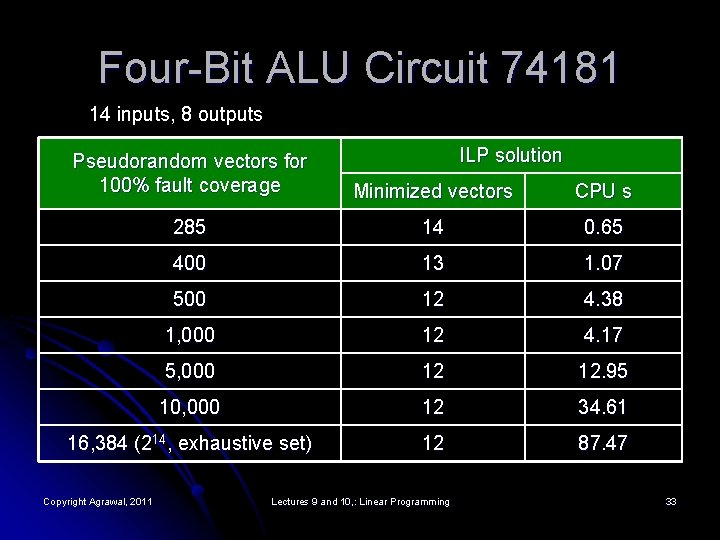
Four-Bit ALU Circuit 74181 14 inputs, 8 outputs ILP solution Pseudorandom vectors for 100% fault coverage Minimized vectors CPU s 285 14 0. 65 400 13 1. 07 500 12 4. 38 1, 000 12 4. 17 5, 000 12 12. 95 10, 000 12 34. 61 16, 384 (214, exhaustive set) 12 87. 47 Copyright Agrawal, 2011 Lectures 9 and 10, : Linear Programming 33

Finding LP/ILP Solvers l l l R. Fourer, D. M. Gay and B. W. Kernighan, AMPL: A Modeling Language for Mathematical Programming, South San Francisco, California: Scientific Press, 1993. Several of programs described in this book are available to Auburn users. B. R. Hunt, R. L. Lipsman, J. M. Rosenberg, K. R. Coombes, J. E. Osborn and G. J. Stuck, A Guide to MATLAB for Beginners and Experienced Users, Cambridge University Press, 2006. Search the web. Many programs with small number of variables can be downloaded free. Copyright Agrawal, 2011 Lectures 9 and 10, : Linear Programming 34

A Circuit Optimization Problem l Given: l Circuit netlist l Cell library with multiple versions for each cell l Select cell versions to optimize a specified characteristic of the circuit. Typical characteristics are: l Area l Power l Delay l Example: Minimize power for given delay. Copyright Agrawal, 2011 Lectures 9 and 10, : Linear Programming 35

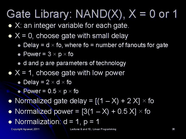
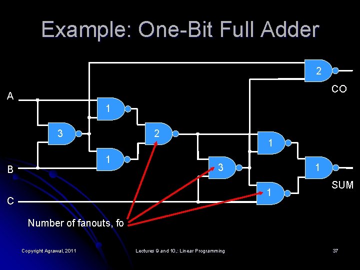
Gate Library: NAND(X), X = 0 or 1 l l X: an integer variable for each gate. X = 0, choose gate with small delay l l X = 1, choose gate with low power l l l Delay = d × fo, where fo = number of fanouts for gate Power = 3 × p × fo d and p are parameters of technology Delay = 2 × d × fo Power = 0. 5 × p × fo Normalized gate delay = [(1 – X) + 2 X] × fo Normalized power = [3(1 – X) + 0. 5 X] × fo Normalization: d = 1, p = 1 Copyright Agrawal, 2011 Lectures 9 and 10, : Linear Programming 36

Example: One-Bit Full Adder 2 CO A 1 3 2 1 B 1 3 1 1 C SUM Number of fanouts, fo Copyright Agrawal, 2011 Lectures 9 and 10, : Linear Programming 37

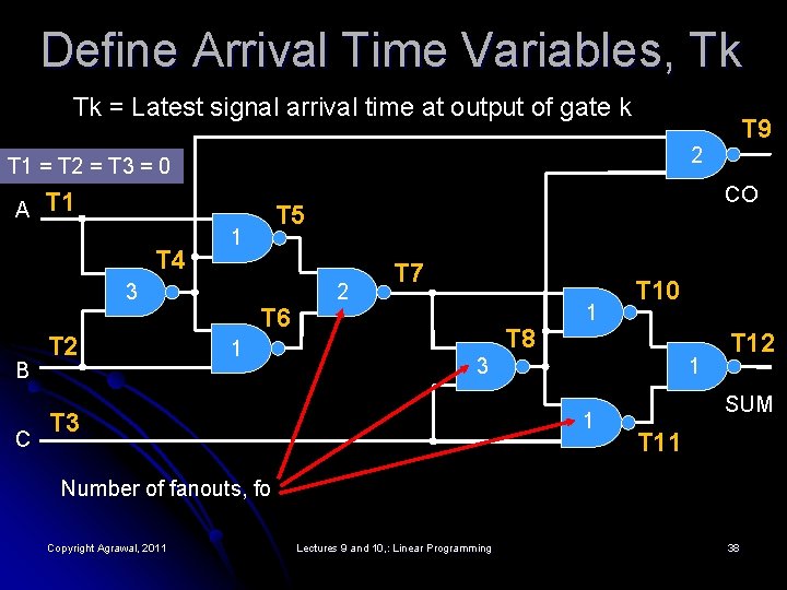
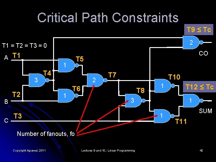
Define Arrival Time Variables, Tk Tk = Latest signal arrival time at output of gate k 2 T 1 = T 2 = T 3 = 0 A T 1 T 4 B C CO T 5 1 3 T 2 T 9 T 6 1 2 T 7 T 8 1 T 10 3 T 3 1 1 T 12 SUM T 11 Number of fanouts, fo Copyright Agrawal, 2011 Lectures 9 and 10, : Linear Programming 38

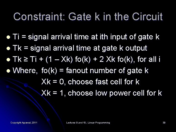
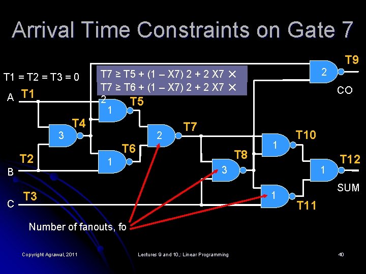
Constraint: Gate k in the Circuit Ti = signal arrival time at ith input of gate k l Tk = signal arrival time at gate k output l Tk ≥ Ti + (1 – Xk) fo(k) + 2 Xk fo(k), for all i l Where, fo(k) = fanout number of gate k Xk = 0, choose fast cell for k Xk = 1, choose low power cell for k l Copyright Agrawal, 2011 Lectures 9 and 10, : Linear Programming 39

Arrival Time Constraints on Gate 7 T 1 = T 2 = T 3 = 0 A T 1 3 T 2 B C 2 T 7 ≥ T 5 + (1 – X 7) 2 + 2 X 7 ✕ 2 T 7 ≥ T 6 + (1 – X 7) 2 + 2 X 7 ✕ 2 T 5 1 T 4 2 1 CO T 7 T 6 T 8 1 T 10 3 T 9 1 1 T 12 SUM T 11 Number of fanouts, fo Copyright Agrawal, 2011 Lectures 9 and 10, : Linear Programming 40

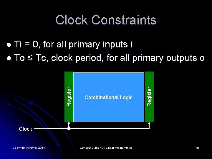
Clock Constraints Ti = 0, for all primary inputs i l To ≤ Tc, clock period, for all primary outputs o Combinational Logic Register l Clock Copyright Agrawal, 2011 Lectures 9 and 10, : Linear Programming 41

Critical Path Constraints T 9 ≤ Tc 2 T 1 = T 2 = T 3 = 0 A T 1 T 5 1 3 B C T 4 T 2 CO 2 1 T 7 T 10 T 6 T 8 1 T 12 ≤ Tc 3 T 3 1 1 SUM T 11 Number of fanouts, fo Copyright Agrawal, 2011 Lectures 9 and 10, : Linear Programming 42

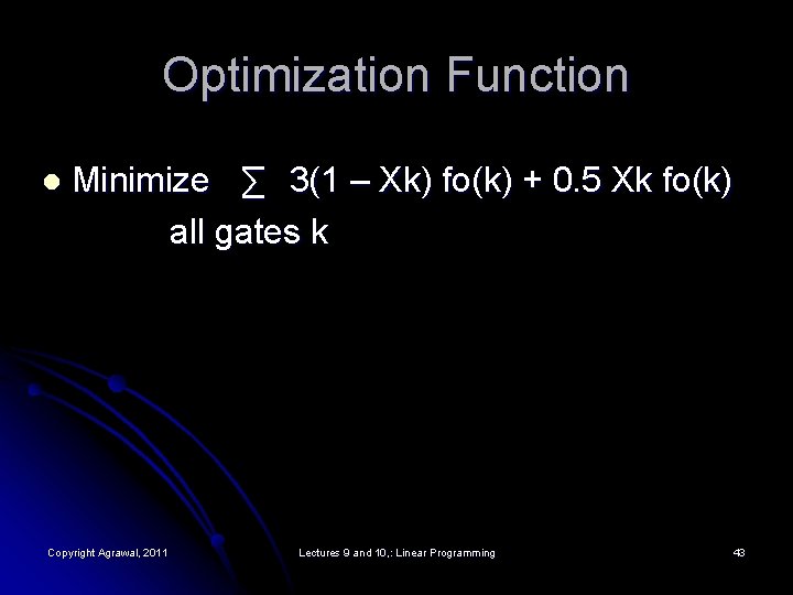
Optimization Function l Minimize ∑ 3(1 – Xk) fo(k) + 0. 5 Xk fo(k) all gates k Copyright Agrawal, 2011 Lectures 9 and 10, : Linear Programming 43

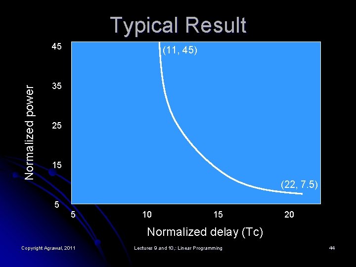
Typical Result Normalized power 45 (11, 45) 35 25 15 (22, 7. 5) 5 5 10 15 20 Normalized delay (Tc) Copyright Agrawal, 2011 Lectures 9 and 10, : Linear Programming 44