Lossless Compression Multimedia Systems Module 2 r Lesson

Lossless Compression Multimedia Systems (Module 2) r Lesson 1: m Minimum Redundancy Coding based on Information Theory: • Shannon-Fano Coding • Huffman Coding r Lesson 2: m Adaptive Coding based on Statistical Modeling: • Adaptive Huffman • Arithmetic coding r Lesson 3: m Dictionary-based Coding • LZW 1

Lossless Compression Multimedia Systems (Module 2 Lesson 1) Summary: r Compression m m r r r With loss Without loss Shannon: Information Theory Shannon-Fano Coding Algorithm Huffman Coding Algorithm Sources: r The Data Compression Book, 2 nd Ed. , Mark Nelson and Jean -Loup Gailly. r Dr. Ze-Nian Li’s course material 2

Compression Why Compression? All media, be it text, audio, graphics or video has “redundancy”. Compression attempts to eliminate this redundancy. What is Redundancy? m m If one representation of a media content, M, takes X bytes and another takes Y bytes(Y< X), then X is a redundant representation relative to Y. Other forms of Redundancy If the representation of a media captures content that is not perceivable by humans, then removing such content will not affect the quality of the content. • For example, capturing audio frequencies outside the human hearing range can be avoided without any harm to the audio’s quality. Is there a representation with an optimal size Z that cannot be improved upon? This question is tackled by information theory. 3

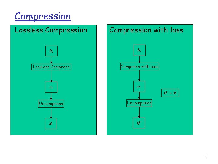
Compression Lossless Compression with loss M M Lossless Compress with loss m m Uncompress M M’ M’ M 4

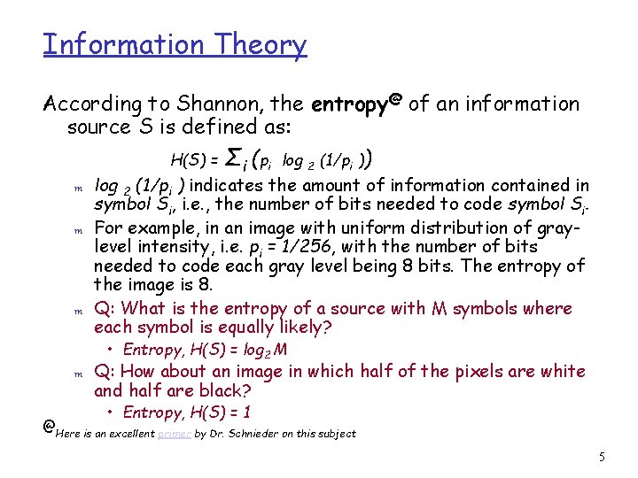
Information Theory According to Shannon, the entropy@ of an information source S is defined as: H(S) = m m m Σi ( p i log 2 (1/pi )) log 2 (1/pi ) indicates the amount of information contained in symbol Si, i. e. , the number of bits needed to code symbol Si. For example, in an image with uniform distribution of graylevel intensity, i. e. pi = 1/256, with the number of bits needed to code each gray level being 8 bits. The entropy of the image is 8. Q: What is the entropy of a source with M symbols where each symbol is equally likely? • Entropy, H(S) = log 2 M m Q: How about an image in which half of the pixels are white and half are black? • Entropy, H(S) = 1 @Here is an excellent primer by Dr. Schnieder on this subject 5

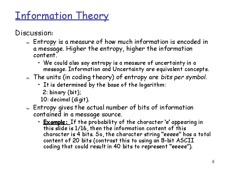
Information Theory Discussion: m Entropy is a measure of how much information is encoded in a message. Higher the entropy, higher the information content. • We could also say entropy is a measure of uncertainty in a message. Information and Uncertainty are equivalent concepts. m The units (in coding theory) of entropy are bits per symbol. m Entropy gives the actual number of bits of information contained in a message source. • It is determined by the base of the logarithm: 2: binary (bit); 10: decimal (digit). • Example: If the probability of the character ‘e’ appearing in this slide is 1/16, then the information content of this character is 4 bits. So, the character string “eeeee” has a total content of 20 bits (contrast this to using an 8 -bit ASCII coding that could result in 40 bits to represent “eeeee”). 6

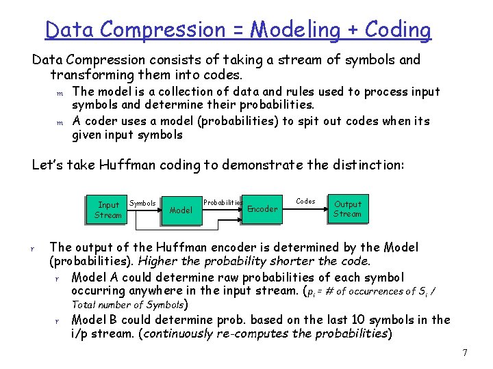
Data Compression = Modeling + Coding Data Compression consists of taking a stream of symbols and transforming them into codes. m m The model is a collection of data and rules used to process input symbols and determine their probabilities. A coder uses a model (probabilities) to spit out codes when its given input symbols Let’s take Huffman coding to demonstrate the distinction: Input Symbols Stream r Model Probabilities Encoder Codes Output Stream The output of the Huffman encoder is determined by the Model (probabilities). Higher the probability shorter the code. r Model A could determine raw probabilities of each symbol occurring anywhere in the input stream. (pi = # of occurrences of Si / Total number of Symbols) r Model B could determine prob. based on the last 10 symbols in the i/p stream. (continuously re-computes the probabilities) 7

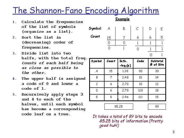
The Shannon-Fano Encoding Algorithm 1. 2. 3. 4. 5. Example Calculate the frequencies of the list of symbols Symbol A B C D E (organize as a list). Count Sort the list in 6 6 5 15 7 (decreasing) order of 0 0 1 1 1 frequencies. 0 1 1 1 0 Divide list into two 1 0 halfs, with the total freq. Symbol Count Info. Code Subtotal Counts of each half being # of Bits -log 2(pi) as close as possible to A 15 1. 38 00 30 the other. x B 7 2. 48 01 14 The upper half is assigned x a code of 0 and lower a C 6 2. 70 10 12 x code of 1. D 6 2. 70 110 18 x Recursively apply steps 3 E 5 2. 96 111 15 and 4 to each of the x halves, until each symbol 85. 25 89 has become a corresponding code leaf on a tree. It takes a total of 89 bits to encode 85. 25 bits of information (Pretty good huh!) 8

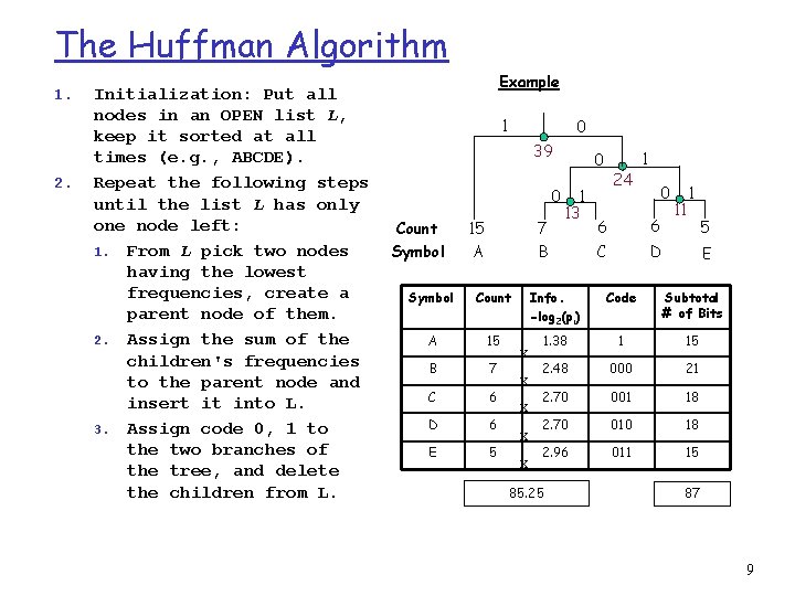
The Huffman Algorithm 1. 2. Initialization: Put all nodes in an OPEN list L, keep it sorted at all times (e. g. , ABCDE). Repeat the following steps until the list L has only one node left: 1. From L pick two nodes having the lowest frequencies, create a parent node of them. 2. Assign the sum of the children's frequencies to the parent node and insert it into L. 3. Assign code 0, 1 to the two branches of the tree, and delete the children from L. Example 1 0 39 0 Count Symbol 15 A 7 B Symbol Count A 15 B 7 C 6 D 6 E 5 x x x 0 1 13 24 1 0 6 6 C D 11 1 5 E Info. -log 2(pi) Code Subtotal # of Bits 1. 38 1 15 2. 48 000 21 2. 70 001 18 2. 70 010 18 2. 96 011 15 85. 25 87 9

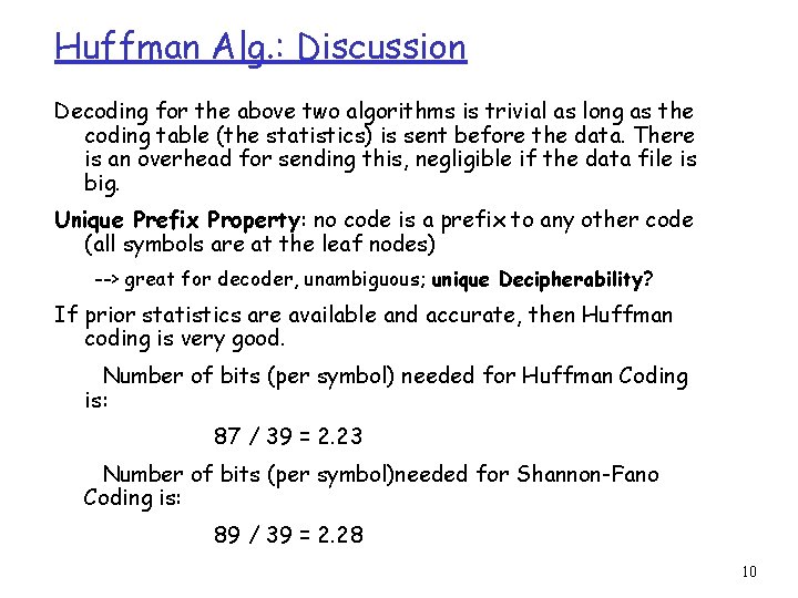
Huffman Alg. : Discussion Decoding for the above two algorithms is trivial as long as the coding table (the statistics) is sent before the data. There is an overhead for sending this, negligible if the data file is big. Unique Prefix Property: no code is a prefix to any other code (all symbols are at the leaf nodes) --> great for decoder, unambiguous; unique Decipherability? If prior statistics are available and accurate, then Huffman coding is very good. Number of bits (per symbol) needed for Huffman Coding is: 87 / 39 = 2. 23 Number of bits (per symbol)needed for Shannon-Fano Coding is: 89 / 39 = 2. 28 10