LongPeriod Seismometry Jonathan Berger Institute of Geophysics and

Long-Period Seismometry Jonathan Berger Institute of Geophysics and Planetary Physics Scripps Institution of Oceanography University of California San Diego

Basics v Measure motion of Earth’s surface relative to some inertial reference frame v Applied to a mass-on-a-spring suspension, in the Laplace domain:

v For frequencies much smaller than the resonant frequency, w 0 , mass position is proportional to ground acceleration. v The smaller the resonant frequency the larger the mass motion for a given ground acceleration.

WHAT ARE THE REQUIRMENTS? v What do we want to measure SIGNALS v How accurately do we want to measure – RESOLUTION v Over what frequencies do we want to measure - BANDWIDTH

What Bandwidth is Required v Gravest Normal Mode – 0. 3 m. Hz v Top end of Teleseismic signals ~ 1 Hz v Top end of Regional Signals ~ 10 Hz v Top end of Strong Motion ~ 30 Hz

WHAT IS THE REQUIRED RESOLUTION? v WHAT IS THE EARTH’S AMBIENT NOISE FIELD? v LOOK AT LOWEST OBSERVED NOISE LEVELS TO ESTIMATE REQUIRED RESOLUTION - A MOVING TARGET

NOISE

Brune & Oliver, 1959 “There are virtually no data on noise in the range of periods between 20 seconds and the earth tide periods. ”

Melton, 1976
")
Agnew & Berger (1978)
")
Peterson 1993 (aka USGS NLNM)

Routine Noise Estimation

Evolution of Noise Models
/Hz Which at long periods corresponds")
Want to resolve 4 x 10 -20(m 2 s-4)/Hz Which at long periods corresponds to rms. mass displacement = 5 x-12 * P 02 m/√Hz [Radius of H atom ~ 4 x 10 -11 m]

Thermal Issues v Thermal noise of a damped harmonic oscillator v Thermal expansion of seismometer suspension v Thermoelastic effect of seismometer spring v Environmental protection

Where K – Boltzmans Constant T – Temperature in Kelvin degrees ~ 290 K˚ m – Mass (kg), P 0 – Free Period (s) Q – Quality Factor of spring (damping) Example, m= 0. 5 kg, P 0 = 10 s, Q= ½ m. P 0 Q = 2. 5 Thermal Noise = 4 x 10 -20 (ms-2)2/Hz

v. Temp coefficient of seismometer “material” > 10 -5/C˚ v. Want to resolve long-period accelerations ~ 10 -11 ∂g/g Implies temperature stability ~ 1 µC˚ v How to get µC˚ temperature stability? v Thermostating is impractical. v Want to minimize seismometer’s ability to exchange thermal energy with its surroundings. v Vault, borehole, enclosure, …
 is temperature as a function of time")
Where u = u(t, x, y, z) is temperature as a function of time and space. - Thermal Diffusivity in m 2/s = / cp Substances with high thermal diffusivity rapidly adjust their temperature to that of their surroundings, because they conduct heat quickly in comparison to their volumetric heat capacity or 'thermal bulk'. - Thermal conductivity in W/m. K˚ cp – Volumetric Heat Capacity in J/m 3. K˚

Thermal Time Constant The time constant for heat applied at the surface of a 1 D insulating body with thermal diffusivity to penetrate a distance L

STS 1 Suspension v Spring is a bi-metal structure designed to reduce temperature effects. v Observed TC of suspension ~ 3. 5 x 10 -5 m/C˚or, with a free period of 20 s ~ 4. 5 x 10 -6 ms-2/C˚ v To resolve long-period rms of 10 -10 ms-2 we need long-period temperature stability of ~20 µC˚

Temperature in the Pinon Flat Observatory Vault

5 x 10 -5 5 x 10 -7 5 x 10 -8 5 x 10 -9 Target 10 -10 ms-2 5 x 10 -10 5 x 10 -11 Acceleration ms-2/√Hz 5 x 10 -6

SIGNALS

Earthscope - Permanent Array Prior to 1969 there were only a handful of Normal Mode observations, all from earthquakes > Mw 8. 5

1970 Columbia Earthquake Mw 8. 0 produced first observations of mode overtones using La. Coste gravimeters modified with feedback for electronic recording.

Now routine processing Mw > 6. 6

Earth Hummmmm v In 1998, almost forty years after the initial attempt by Benioff et al (1959), continuous free oscillations of the Earth were finally observed. v Earth is constantly excited by spheroidal fundamental modes between about 2 and 7 m. Hz (from 0 S 15 to 0 S 60) with nearly constant acceleration and are about 3 – 5 x 10 -12 ms-2.

Period: 0. 3 to 10 m. Hz Amplitudes: to ~10 -5 ms-2 (“Slichter” Mode: 35 – 70 µHz ? ) Normal Modes

Sources >_ 3000 km Period: a few m. Hz to several Hz Amplitudes: to ~10 -3 ms-2

Sources >_ 100 km Period: a few 10’s s to ~10 Hz Amplitudes: to ~10 -1 ms-2

Lg Phase observed at PFO, M 6. 9, Distance 630 Km Clip Level

Sources >~10 km Period: a few seconds to ~30 Hz Amplitudes: to ~10 ms-2

220 d. B

Instruments

Feedback Model Ground Acceleration Suspension Mass Motion Displacement Xducer Mass forced to oppose ground acceleration Forcer Feedback Controller Acceleration √elocity

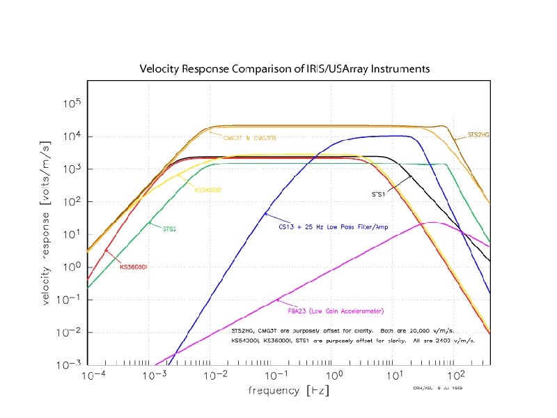
Commercial Broadband Seismometers

STS 1 with bell jar KS 54000 ready to go down WRAB Borehole

Trillium 240 CMG-3 T STS-2

Some Features of the New version STS-1 v Non-Galperin: Separate H and V Sensor Designs v Factory-Leveled: Plug and Go in Leveled Package v 360 Second to 15 Hz Passband v Self-Noise Comparable to Original Sensors v Incorporates Wielandt/ASL “Warpless Baseplate” Design v Three Aluminum Vacuum Chambers on Single Baseplate; All-Metal Valve v Integrated Magnetic Shield for V Sensor v Galvanic Isolation from Pier See Poster by Van. Zandt

Interferometric Seismometer v Interferometric Displacement Transducer v Large Bandwidth & Dynamic Range v No Feedback; No enclosed electronics; No Electrical Connections v Capable of operating in extreme temperatures See Poster by Otero et al.

Station Requirements for Long Period Observations v Good thermal stability v Solid rock foundations for local tilt suppression v Far from coast (Yet island stations are required) v Human Factor ….

The GSN Station PALK 100 m, steel-cased, Borehole

The GSN Station AAK The tunnel entrance The GSN Station AAK One of the vaults

DGAR - Vault under construction

Final Thoughts v Modern Broadband Seismometer are pretty good. What more would we like? v Additional Bandwidth – long period end v Reduced long-period noise – small market v Improved environmental protection v Long-term, telemetered, Ocean-bottom instruments


GSN Station UOSS

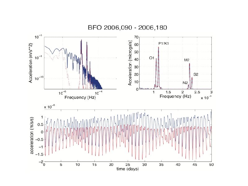
Nature’s Calibration Signal: Earth Tides

Effect of increasing mass in Superconducting Gravimeter
 & New(1993) Noise Models")
USGS Old (1980) & New(1993) Noise Models

DGAR - Inside the Vault

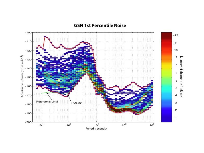
Berger et al. , 2003 v 118 GSN Stations of the IU and II networks for the year July 2001 through June 2002. v Each station-channel data segmented into hourly, 1 to 11 hour segments. v noise estimated in 50% overlapping 1/7 decade (∂f/f=0. 33, ~1/2 octave) bands.

Features of Feedback v Limits the dynamic range and linearity requirements of the displacement transducer as the test-mass displacement is reduced by gain of feedback loop v Can easily shape overall response to compensate for suspension free period and Q v Can provide electrical outputs proportional to displacement, velocity, or acceleration
- Slides: 56