Longitudinal design and data management analysis A demonstration

Longitudinal design and data management / analysis A demonstration Mei-kuang Chen EGAD, Department of Psychology, University of Arizona, Tucson, AZ

Experiences – � Program evaluation vs. research � Why demonstration? Data analyst vs. methodologist - How many of you do data analysis yourself? Purpose -> bridge � Data management and analysis � Your experiences? SPSS, R, SAS

Why longitudinal data? � One � Era of best ways to establish cause-effect of Data Explosion – data are available � Good research design – theme of AEA

� SPSS What’s involved in this demonstration? and R – not live demo here � Look at the data and think about the data together - Conceptual level discussion � All the syntax and data files will be shared via a link on Dropbox: Link: https: //www. dropbox. com/sh/39 ix 8 upwgu 0 a wc 6/AADs. SEu. Wshky 6 szic. Kl 62 Hp. Ha? dl=0

Advantages of SPSS � Dropdown menu for restructuring the data � ‘paste’ as an easy way to get the syntax � Always use syntax- paper trail!!

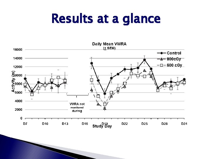
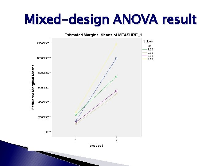
What do we usually do with longitudinal data? � Paired t-test : almost always � Background: Collaborator in NIH need some help with a reviewer’s comment on an animal model in fatigue � The analyses they did: Paired t-test and one-way ANOVA � Reviewer: Paired t-test vs. mixed-design ANOVA (General linear model) � What can be the potential problems for paired t-test?

Results at a glance

Mixed-design ANOVA result

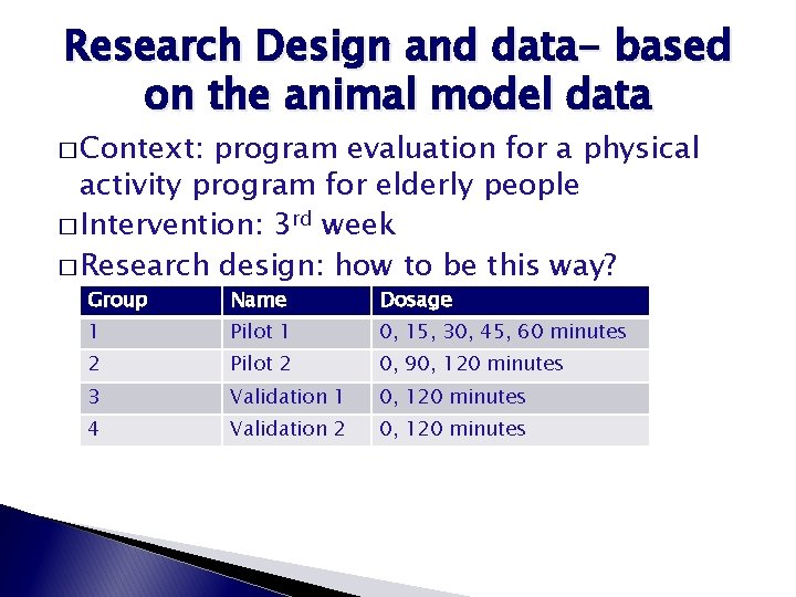
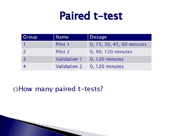
Research Design and data- based on the animal model data � Context: program evaluation for a physical activity program for elderly people � Intervention: 3 rd week � Research design: how to be this way? Group Name Dosage 1 Pilot 1 0, 15, 30, 45, 60 minutes 2 Pilot 2 0, 90, 120 minutes 3 Validation 1 0, 120 minutes 4 Validation 2 0, 120 minutes

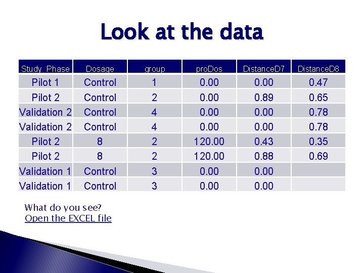
Look at the data Study_Phase Dosage group pro. Dos Distance. D 7 Distance. D 8 Pilot 1 Pilot 2 Validation 2 Pilot 2 Validation 1 Control 8 8 Control 1 2 4 4 2 2 3 3 0. 00 120. 00 0. 89 0. 00 0. 43 0. 88 0. 00 0. 47 0. 65 0. 78 0. 35 0. 69 What do you see? Open the EXCEL file

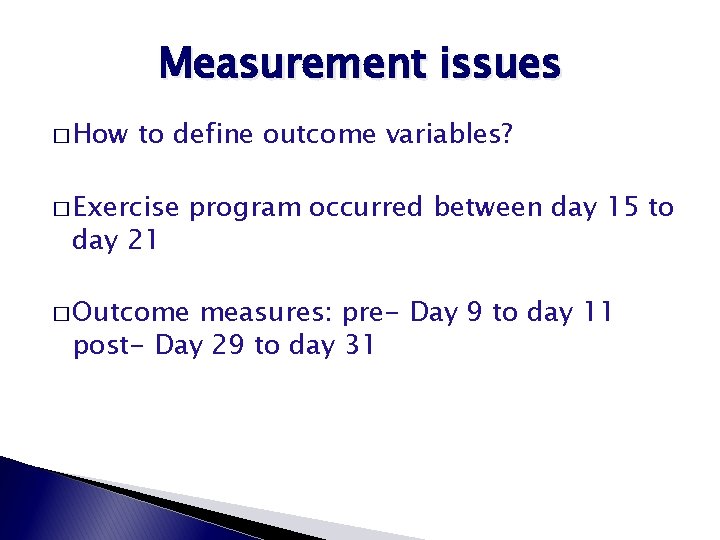
Measurement issues � How to define outcome variables? � Exercise day 21 program occurred between day 15 to � Outcome measures: pre- Day 9 to day 11 post- Day 29 to day 31

Measurement

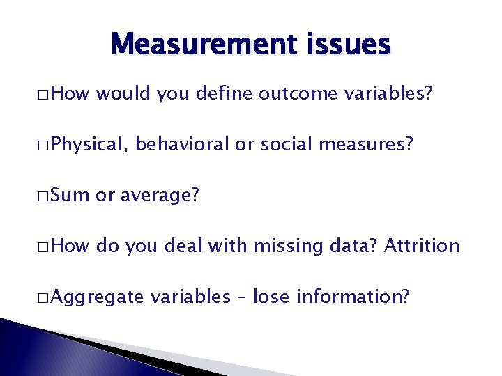
Measurement issues � How would you define outcome variables? � Physical, behavioral or social measures? � Sum or average? � How do you deal with missing data? Attrition � Aggregate variables – lose information?

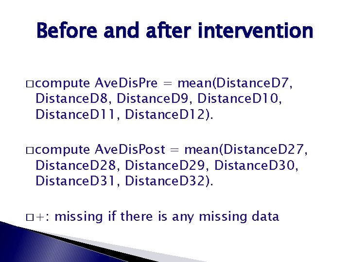
Before and after intervention � compute Ave. Dis. Pre = mean(Distance. D 7, Distance. D 8, Distance. D 9, Distance. D 10, Distance. D 11, Distance. D 12). � compute Ave. Dis. Post = mean(Distance. D 27, Distance. D 28, Distance. D 29, Distance. D 30, Distance. D 31, Distance. D 32). � +: missing if there is any missing data

Paired t-test � How many paired t-tests?

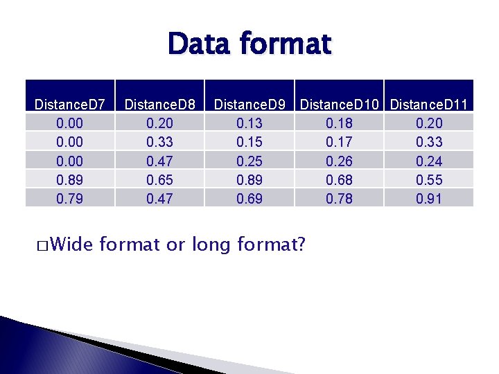
Data format Distance. D 7 0. 00 0. 89 0. 79 � Wide Distance. D 8 0. 20 0. 33 0. 47 0. 65 0. 47 Distance. D 9 0. 13 0. 15 0. 25 0. 89 0. 69 Distance. D 10 Distance. D 11 0. 18 0. 20 0. 17 0. 33 0. 26 0. 24 0. 68 0. 55 0. 78 0. 91 format or long format?

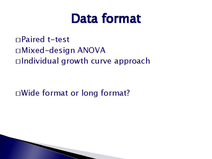
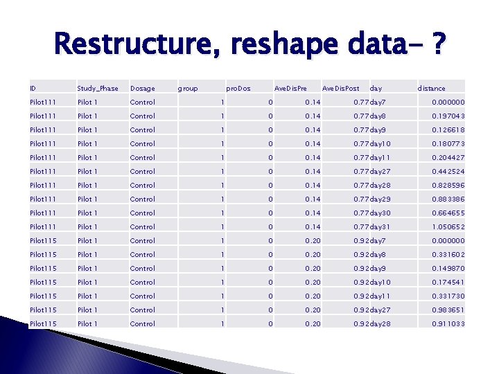
Data format � Paired t-test � Mixed-design ANOVA � Individual growth curve approach � Wide format or long format?

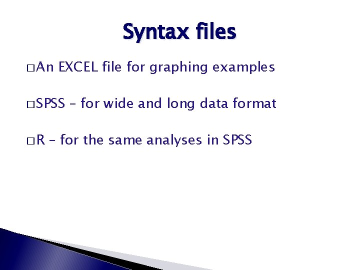
Syntax files � An EXCEL file for graphing examples � SPSS �R – for wide and long data format – for the same analyses in SPSS

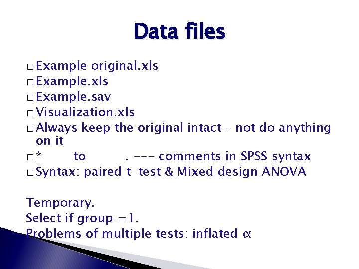
Data files � Example original. xls � Example. sav � Visualization. xls � Always keep the original intact – not do anything on it �* to. --- comments in SPSS syntax � Syntax: paired t-test & Mixed design ANOVA Temporary. Select if group =1. Problems of multiple tests: inflated α

Restructure, reshape data- ? ID Study_Phase Dosage group pro. Dos Ave. Dis. Pre Ave. Dis. Post day distance Pilot 111 Pilot 1 Control 1 0 0. 14 0. 77 day 7 0. 000000 Pilot 111 Pilot 1 Control 1 0 0. 14 0. 77 day 8 0. 197043 Pilot 111 Pilot 1 Control 1 0 0. 14 0. 77 day 9 0. 126618 Pilot 111 Pilot 1 Control 1 0 0. 14 0. 77 day 10 0. 180773 Pilot 111 Pilot 1 Control 1 0 0. 14 0. 77 day 11 0. 204427 Pilot 111 Pilot 1 Control 1 0 0. 14 0. 77 day 27 0. 442524 Pilot 111 Pilot 1 Control 1 0 0. 14 0. 77 day 28 0. 828596 Pilot 111 Pilot 1 Control 1 0 0. 14 0. 77 day 29 0. 883386 Pilot 111 Pilot 1 Control 1 0 0. 14 0. 77 day 30 0. 664655 Pilot 111 Pilot 1 Control 1 0 0. 14 0. 77 day 31 1. 050652 Pilot 115 Pilot 1 Control 1 0 0. 20 0. 92 day 7 0. 000000 Pilot 115 Pilot 1 Control 1 0 0. 20 0. 92 day 8 0. 331602 Pilot 115 Pilot 1 Control 1 0 0. 20 0. 92 day 9 0. 149870 Pilot 115 Pilot 1 Control 1 0 0. 20 0. 92 day 10 0. 174541 Pilot 115 Pilot 1 Control 1 0 0. 20 0. 92 day 11 0. 331730 Pilot 115 Pilot 1 Control 1 0 0. 20 0. 92 day 27 0. 983651 Pilot 115 Pilot 1 Control 1 0 0. 20 0. 92 day 28 0. 911033

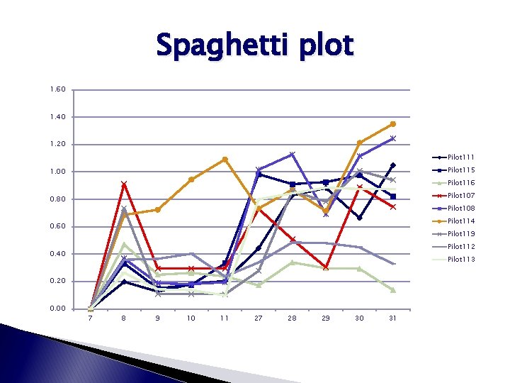
Spaghetti plot 1. 60 1. 40 1. 20 Pilot 111 Pilot 115 1. 00 Pilot 116 Pilot 107 0. 80 Pilot 108 Pilot 114 0. 60 Pilot 119 Pilot 112 0. 40 Pilot 113 0. 20 0. 00 7 8 9 10 11 27 28 29 30 31

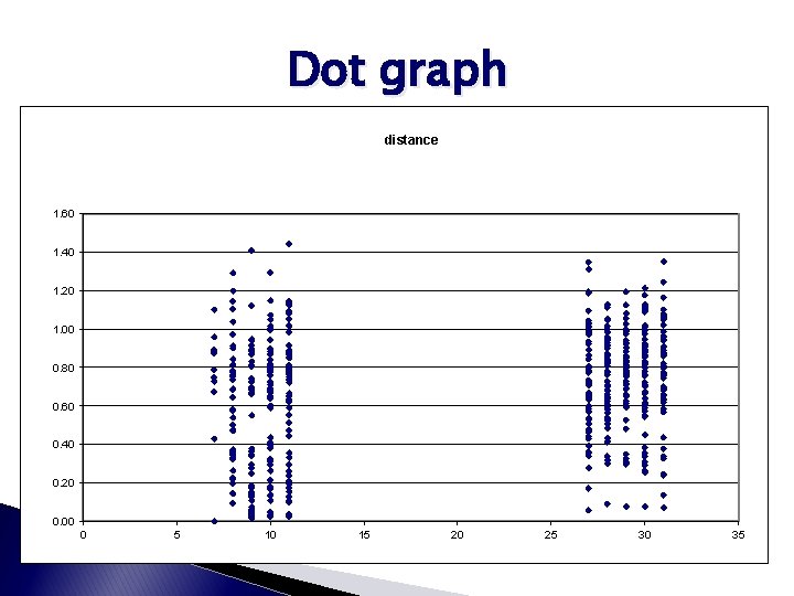
Dot graph distance 1. 60 1. 40 1. 20 1. 00 0. 80 0. 60 0. 40 0. 20 0. 00 0 5 10 15 20 25 30 35

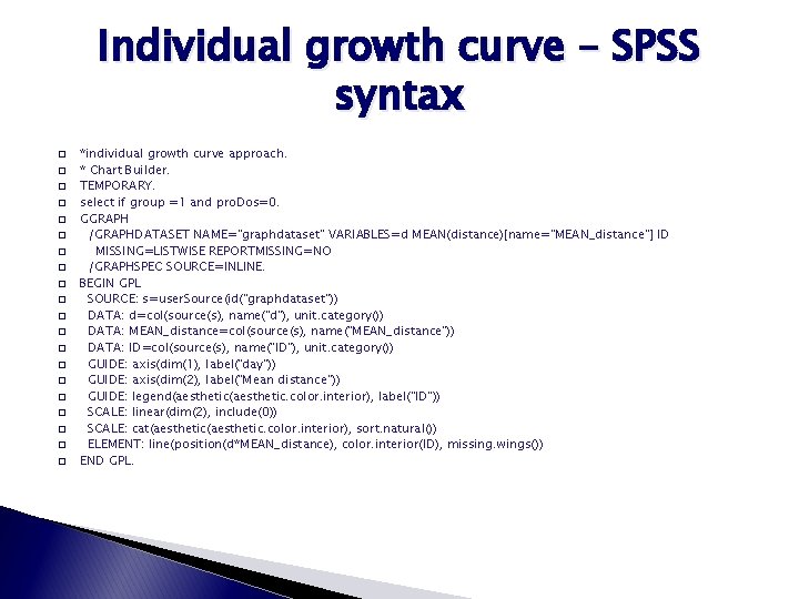
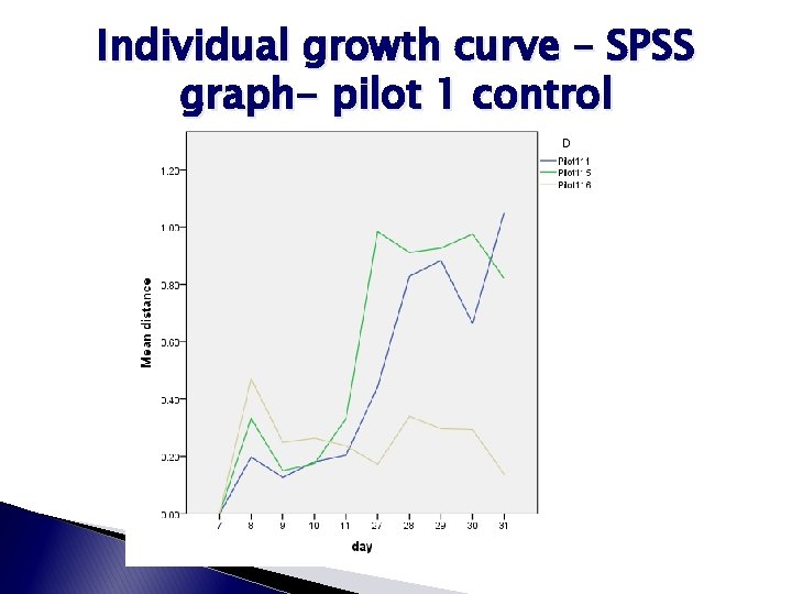
Individual growth curve – SPSS syntax � � � � � *individual growth curve approach. * Chart Builder. TEMPORARY. select if group =1 and pro. Dos=0. GGRAPH /GRAPHDATASET NAME="graphdataset" VARIABLES=d MEAN(distance)[name="MEAN_distance"] ID MISSING=LISTWISE REPORTMISSING=NO /GRAPHSPEC SOURCE=INLINE. BEGIN GPL SOURCE: s=user. Source(id("graphdataset")) DATA: d=col(source(s), name("d"), unit. category()) DATA: MEAN_distance=col(source(s), name("MEAN_distance")) DATA: ID=col(source(s), name("ID"), unit. category()) GUIDE: axis(dim(1), label("day")) GUIDE: axis(dim(2), label("Mean distance")) GUIDE: legend(aesthetic. color. interior), label("ID")) SCALE: linear(dim(2), include(0)) SCALE: cat(aesthetic. color. interior), sort. natural()) ELEMENT: line(position(d*MEAN_distance), color. interior(ID), missing. wings()) END GPL.

Individual growth curve – SPSS graph- pilot 1 control

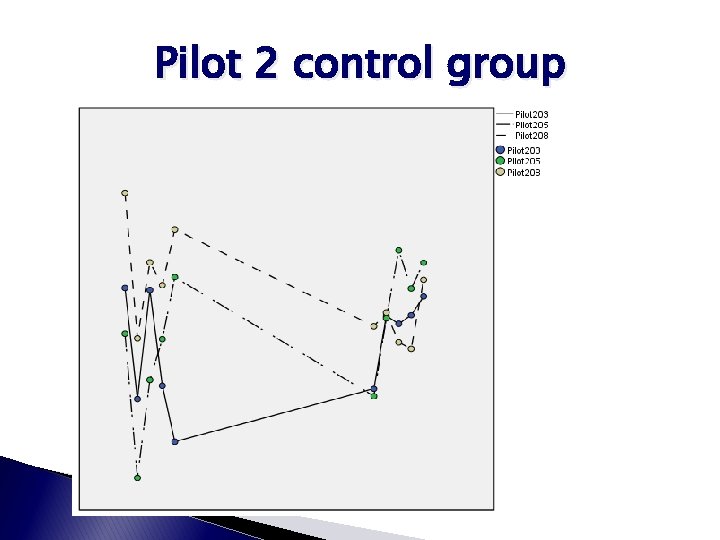
Pilot 2 control group

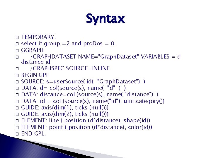
Syntax � � � � TEMPORARY. select if group =2 and pro. Dos = 0. GGRAPH /GRAPHDATASET NAME="Graph. Dataset" VARIABLES = d distance id /GRAPHSPEC SOURCE=INLINE. BEGIN GPL SOURCE: s=user. Source( id( "Graph. Dataset") ) DATA: d= col(source(s), name( "d" ) ) DATA: distance=col (source(s), name( "distance") ) DATA: id = col (source(s), name("id"), unit. category()) GUIDE: axis(dim(1), ticks (null())) GUIDE: axis(dim(2), ticks (null())) ELEMENT: line ( position (d*distance), shape(id)) ELEMENT: point ( position (d*distance), color(id)) END GPL.

Statistical models � Individual growth curve model based on regression � Mixed � SPSS models: time nested within person output file and syntax for the long format data

The same analyses in R �R code: in. R file ◦ # for comments ◦ read in the data first -. csv data or simple text data is the easiest way to import the data ◦ Learn from the syntax – use it as template

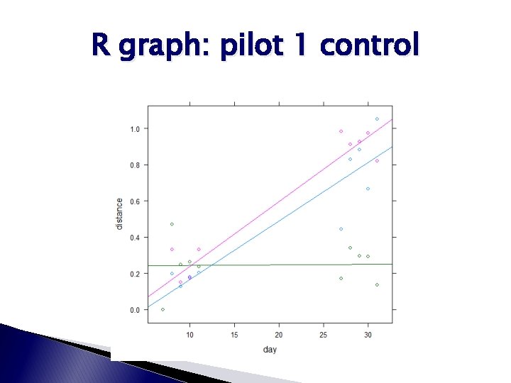
R graph: pilot 1 control

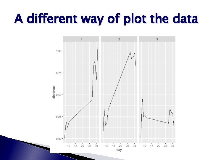
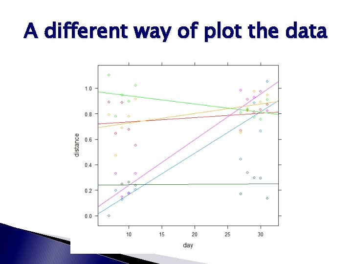
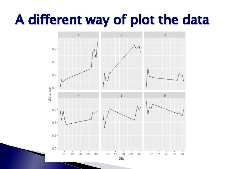
A different way of plot the data

A different way of plot the data

A different way of plot the data

Other approached to longitudinal data analysis � Repeated � Panel cross-sectionals design � Cohort studies � Event history datasets � Time series analyses

Other tools � Latent growth curve model – SEM � Continuous time modeling by Manuel Völkle

Thank you!! � Email: kuang@email. arizona. edu