Long time correlation due to highdimensional chaos in

Long time correlation due to high-dimensional chaos in globally coupled tent map system Tsuyoshi Chawanya Department of Pure and Applied Mathematics, Graduate School of Information Science and Technology, Osaka University (PFDW 05)

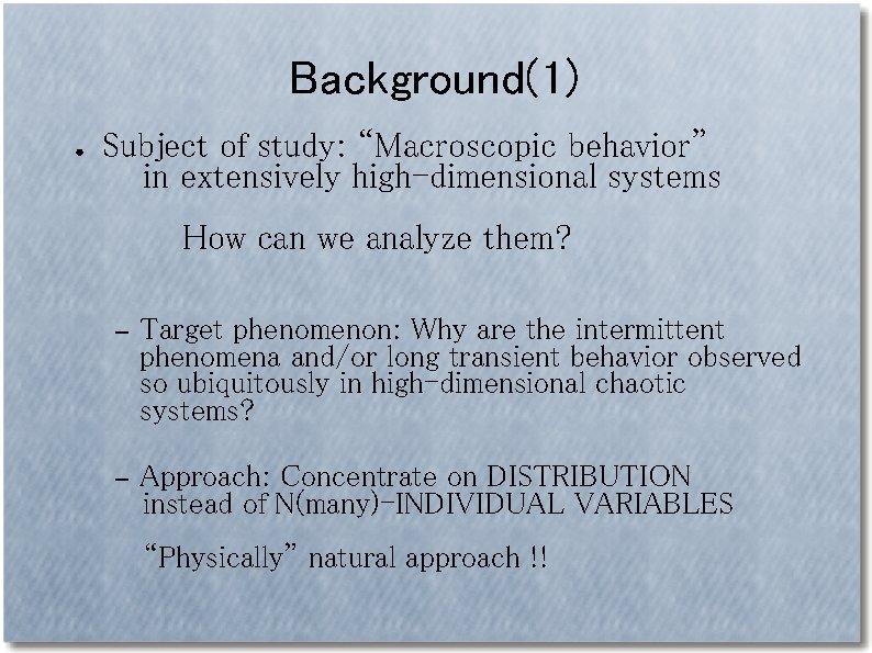
Background(1) ● Subject of study: “Macroscopic behavior” in extensively high-dimensional systems How can we analyze them? – Target phenomenon: Why are the intermittent phenomena and/or long transient behavior observed so ubiquitously in high-dimensional chaotic systems? – Approach: Concentrate on DISTRIBUTION instead of N(many)-INDIVIDUAL VARIABLES “Physically” natural approach !!

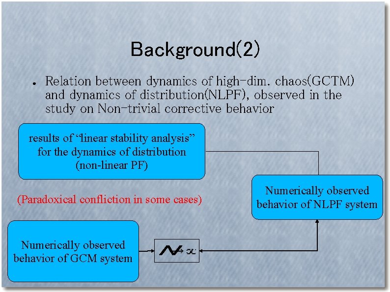
Background(2) ● Relation between dynamics of high-dim. chaos(GCTM) and dynamics of distribution(NLPF), observed in the study on Non-trivial corrective behavior results of “linear stability analysis” for the dynamics of distribution (non-linear PF) (Paradoxical confliction in some cases) Numerically observed behavior of GCM system Numerically observed behavior of NLPF system

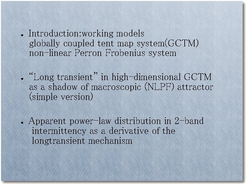
● ● ● Introduction: working models globally coupled tent map system(GCTM) non-linear Perron Frobenius system “Long transient” in high-dimensional GCTM as a shadow of macroscopic (NLPF) attractor (simple version) Apparent power-law distribution in 2 -band intermittency as a derivative of the longtransient mechanism

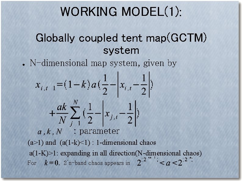
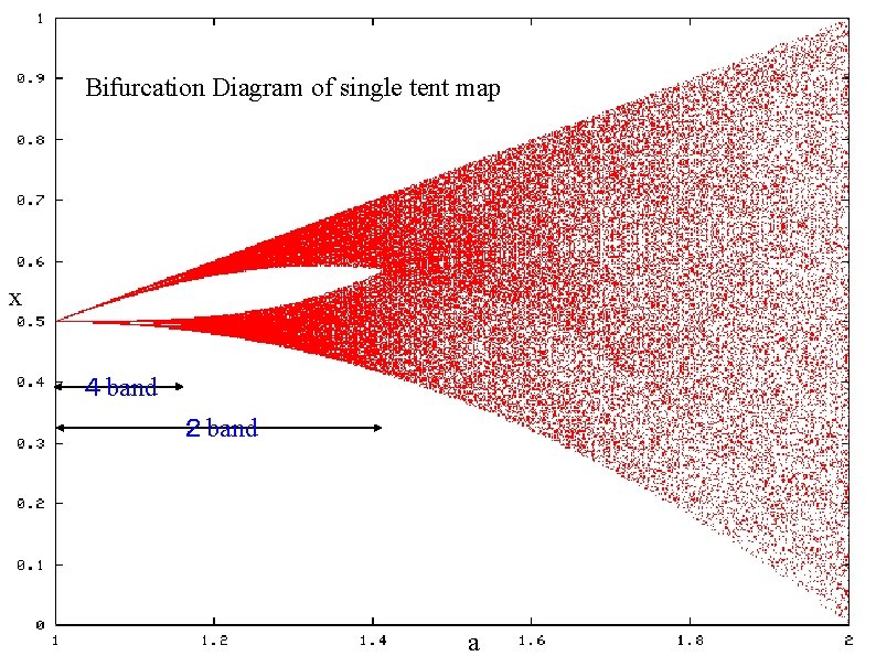
WORKING MODEL(1): Globally coupled tent map(GCTM) system ● N-dimensional map system, given by : parameter (a>1) and (a(1 -k)<1) : 1 -dimensional chaos a(1 -K)>1: expanding in all direction(N-dimensional chaos) For 　　　　 , 2^n-band chaos appears in

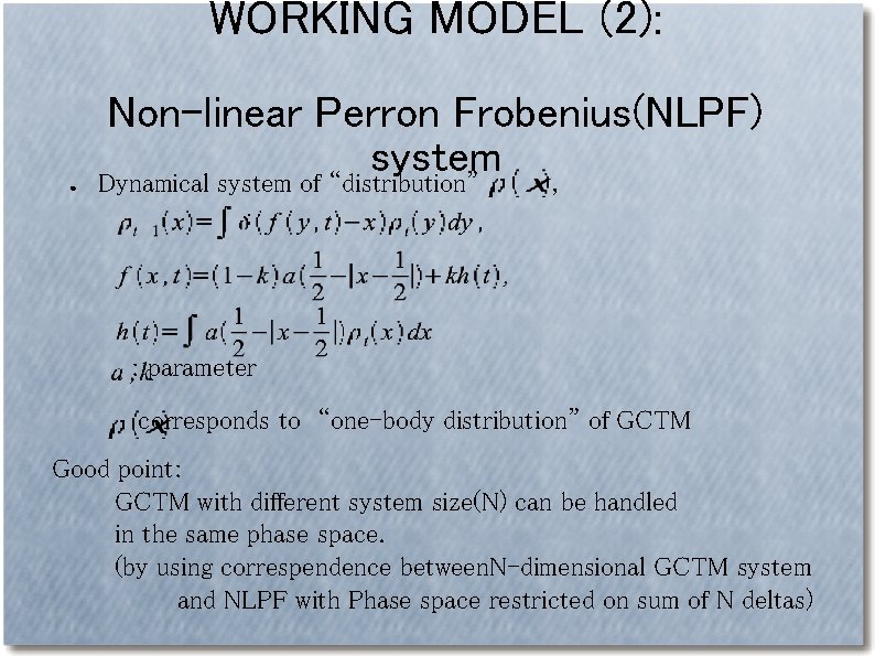
WORKING MODEL (2): ● Non-linear Perron Frobenius(NLPF) system Dynamical system of “distribution” , : parameter corresponds to “one-body distribution” of GCTM Good point: GCTM with different system size(N) can be handled in the same phase space. (by using correspendence between. N-dimensional GCTM system and NLPF with Phase space restricted on sum of N deltas)

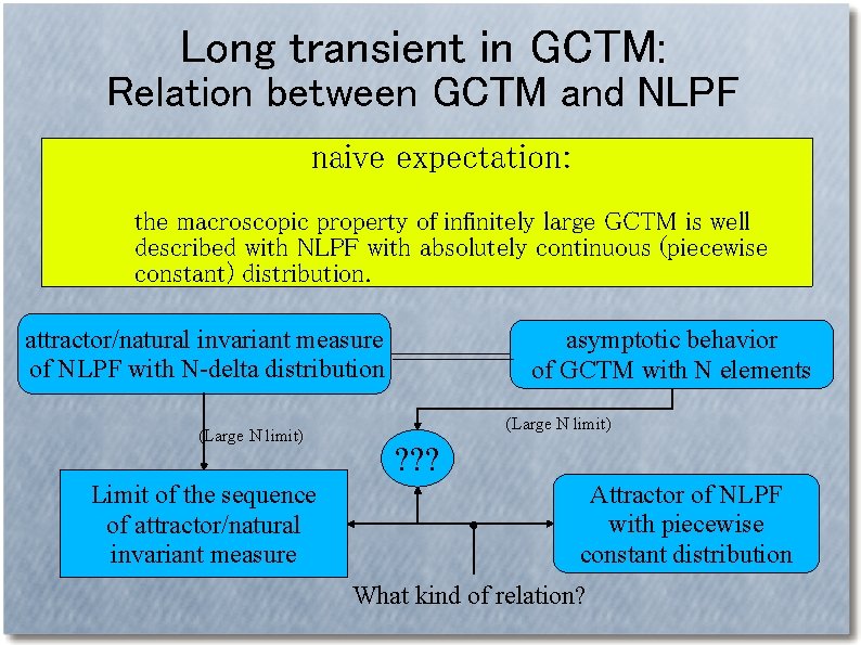
Long transient in GCTM: Relation between GCTM and NLPF naive expectation: thethe macroscopic property of of infinitely large GCTM is is well macroscopic property infinitely large GCTM well described with NLPF with absolutely continuous distribution (piecewise constant distribution). constant) distribution. attractor/natural invariant measure of NLPF with N-delta distribution (Large N limit) Limit of the sequence of attractor/natural invariant measure asymptotic behavior of GCTM with N elements (Large N limit) ? ? ? Attractor of NLPF with piecewise constant distribution What kind of relation?

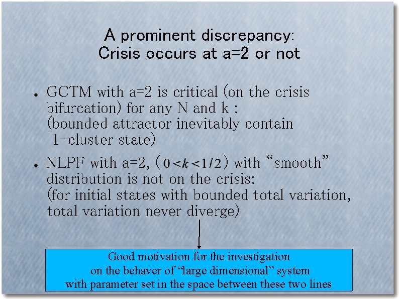
A prominent discrepancy: Crisis occurs at a=2 or not ● ● GCTM with a=2 is critical (on the crisis bifurcation) for any N and k : (bounded attractor inevitably contain 1 -cluster state) NLPF with a=2, ( ) with “smooth” distribution is not on the crisis: (for initial states with bounded total variation, total variation never diverge) Good motivation for the investigation on the behaver of “large dimensional” system with parameter set in the space between these two lines

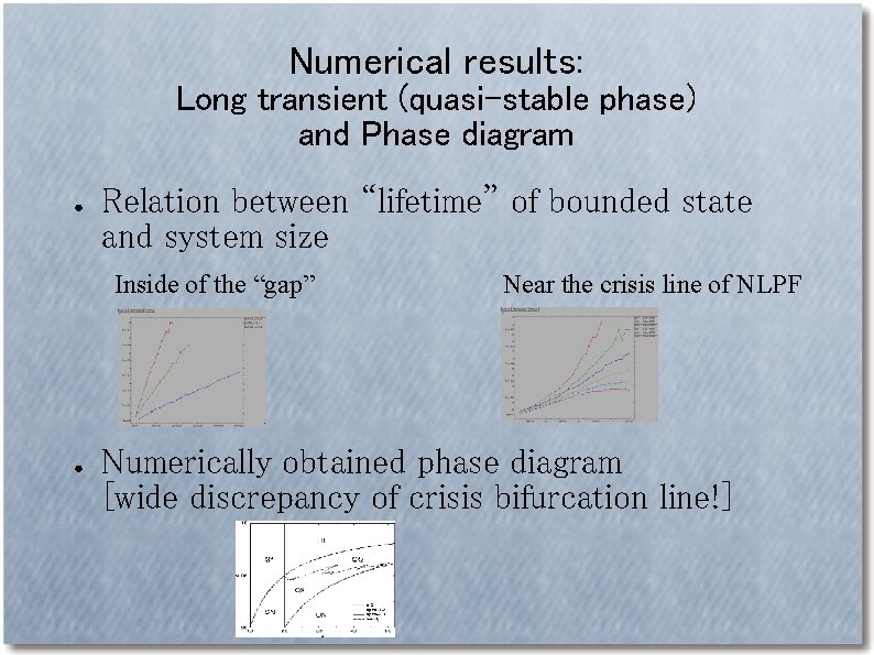
Numerical results: Long transient (quasi-stable phase) and Phase diagram ● Relation between “lifetime” of bounded state and system size Inside of the “gap” ● Near the crisis line of NLPF Numerically obtained phase diagram [wide discrepancy of crisis bifurcation line!]

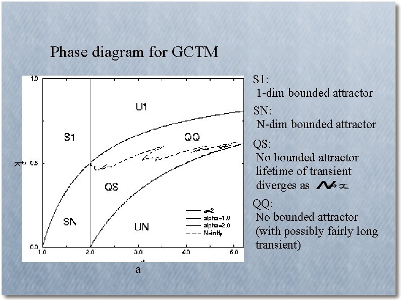
Phase diagram for GCTM S 1: 1 -dim bounded attractor SN: N-dim bounded attractor k QS: No bounded attractor lifetime of transient diverges as. QQ: No bounded attractor (with possibly fairly long transient) a

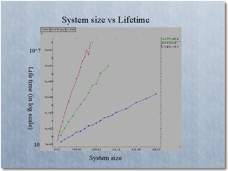
System size vs Lifetime 10^7 Life time (in log scale) 10 System size

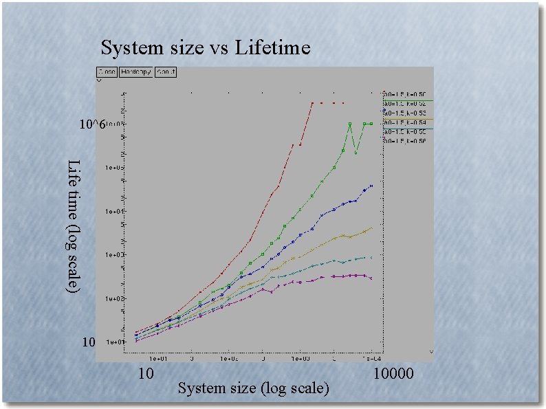
System size vs Lifetime 10^6 Life time (log scale) 10 10 System size (log scale) 10000

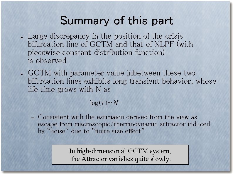
Summary of this part ● ● Large discrepancy in the position of the crisis bifurcation line of GCTM and that of NLPF (with piecewise constant distribution function) is observed GCTM with parameter value inbetween these two bifurcation lines exhibits long transient behavior, whose life time grows with N as – Consistent with the estimaion derived from the view as escape from macroscopic/thermodynamic attractor induced by “noise” due to “finite size effect” In high-dimensional GCTM system, the Attractor vanishes quite slowly.

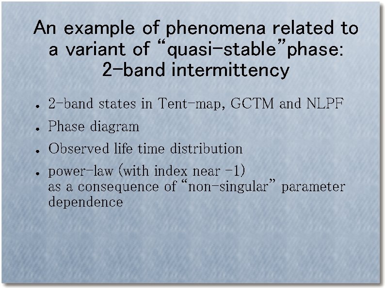
An example of phenomena related to a variant of “quasi-stable”phase: 2 -band intermittency ● ● 2 -band states in Tent-map, GCTM and NLPF Phase diagram Observed life time distribution power-law (with index near -1) as a consequence of “non-singular” parameter dependence

Bifurcation Diagram of single tent map x ４ band ２ band a

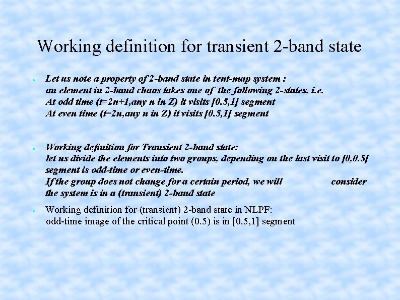
Working definition for transient 2 -band state ● ● ● Let us note a property of 2 -band state in tent-map system : an element in 2 -band chaos takes one of the following 2 -states, i. e. At odd time (t=2 n+1, any n in Z) it visits [0. 5, 1] segment At even time (t=2 n, any n in Z) it visits [0. 5, 1] segment Working definition for Transient 2 -band state: let us divide the elements into two groups, depending on the last visit to [0, 0. 5] segment is odd-time or even-time. If the group does not change for a certain period, we will consider the system is in a (transient) 2 -band state Working definition for (transient) 2 -band state in NLPF: odd-time image of the critical point (0. 5) is in [0. 5, 1] segment

On the stability of 2 -band states ● ● The stability of 2 -band states depends on a, k and the weight ratio of the 2 bands. (no direct dependence on N is observed in numerical calculation) The crysis (band merging) may occur at different point in GCTM and NLPF.

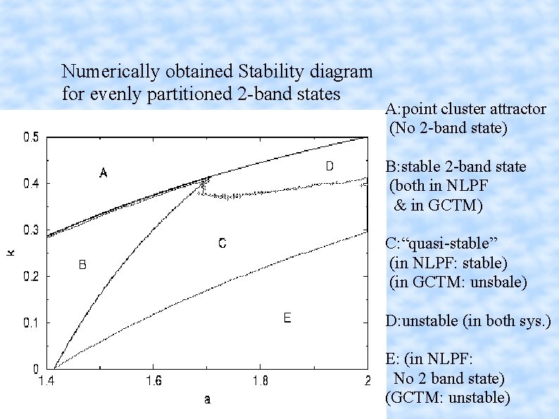
Numerically obtained Stability diagram for evenly partitioned 2 -band states A: point cluster attractor (No 2 -band state) B: stable 2 -band state (both in NLPF & in GCTM) C: “quasi-stable” (in NLPF: stable) (in GCTM: unsbale) D: unstable (in both sys. ) E: (in NLPF: No 2 band state) (GCTM: unstable)

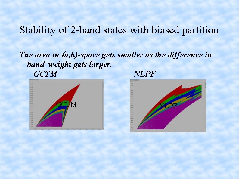
Stability of 2 -band states with biased partition The area in (a, k)-space gets smaller as the difference in band weight gets larger. GCTM NLPF

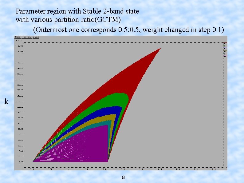
Parameter region with Stable 2 -band state with various partition ratio(GCTM) (Outermost one corresponds 0. 5: 0. 5, weight changed in step 0. 1) k a

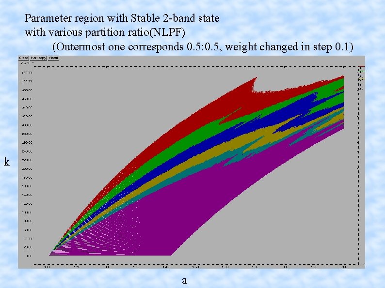
Parameter region with Stable 2 -band state with various partition ratio(NLPF) (Outermost one corresponds 0. 5: 0. 5, weight changed in step 0. 1) k a

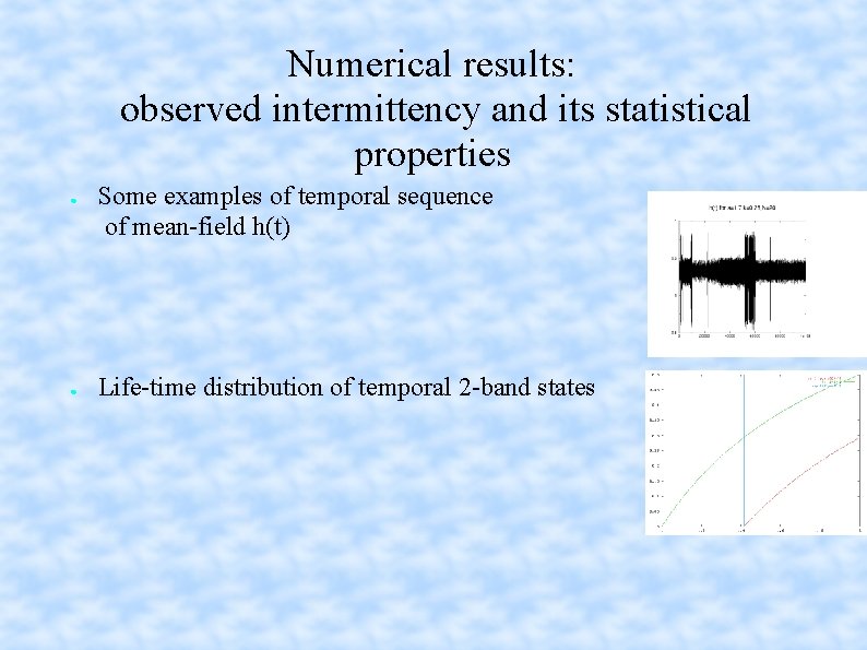
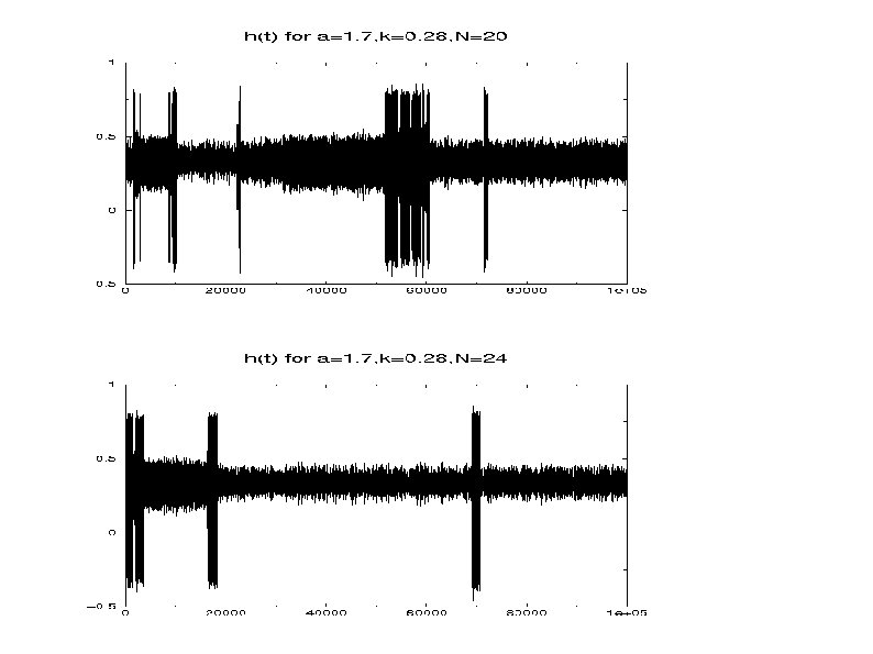
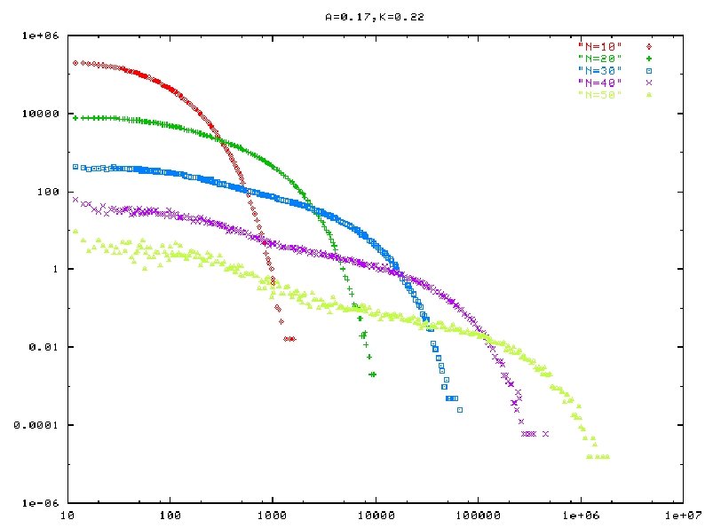
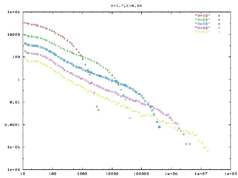
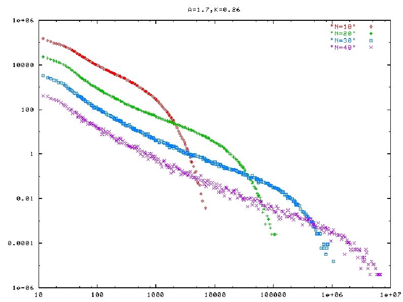
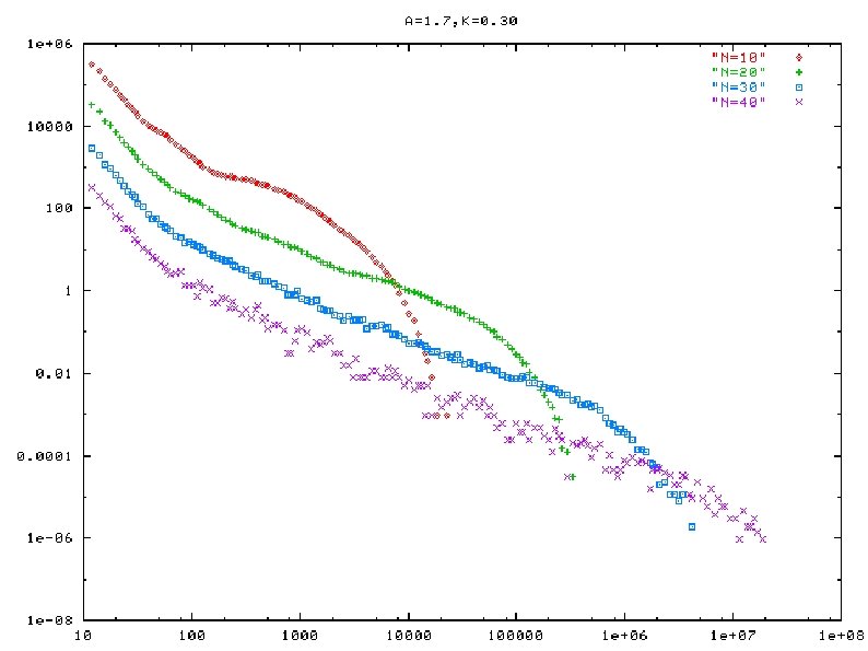
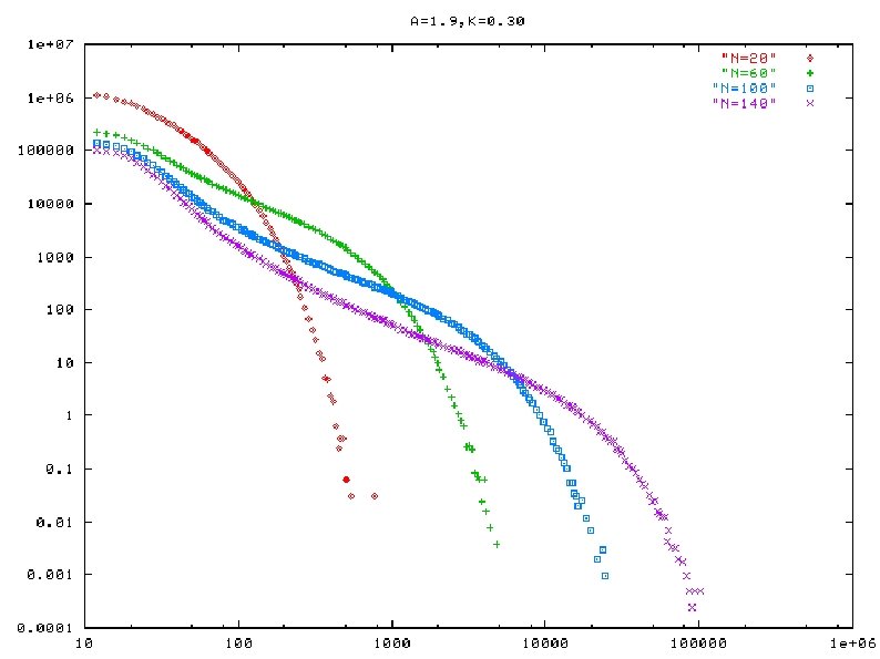
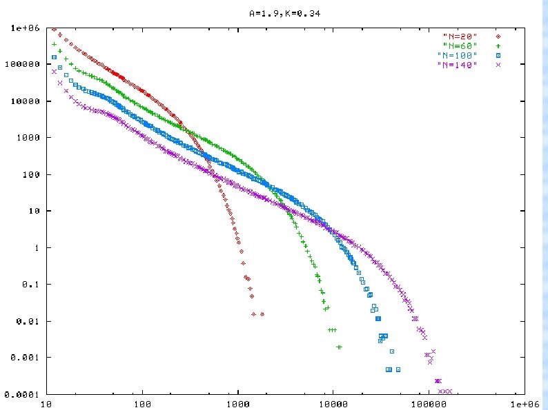
Numerical results: observed intermittency and its statistical properties ● ● Some examples of temporal sequence of mean-field h(t) Life-time distribution of temporal 2 -band states

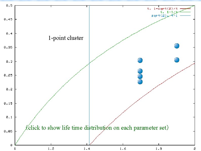
1 -point cluster （click to show life time distribution on each parameter set）

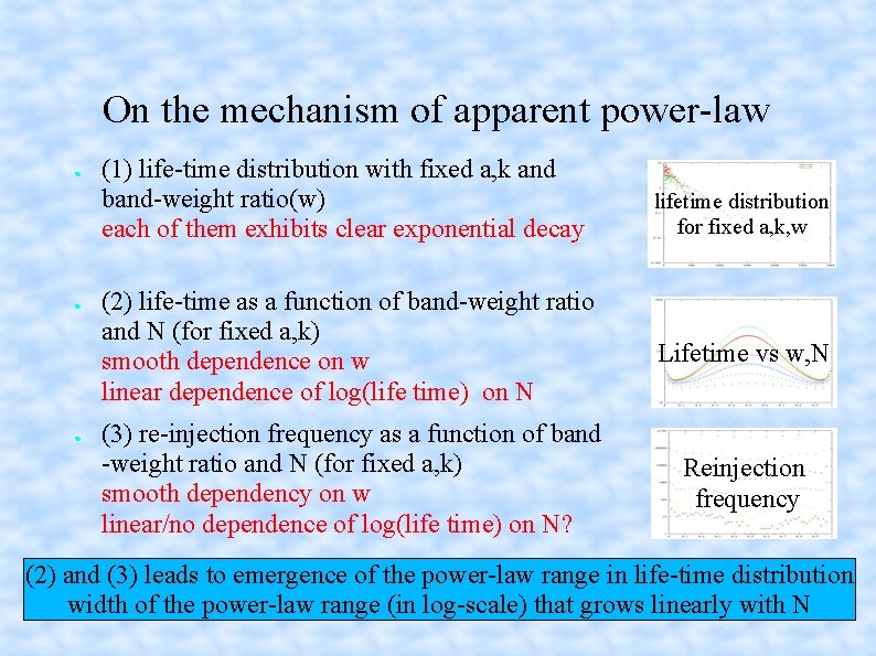
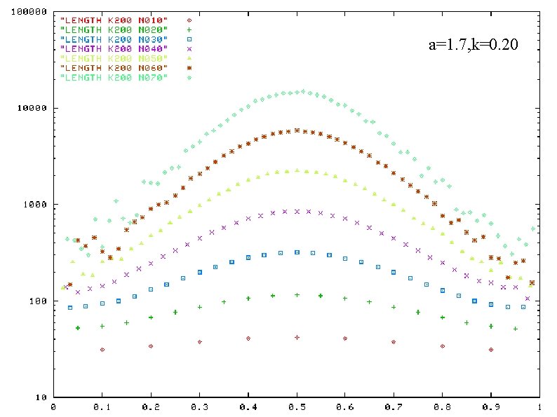
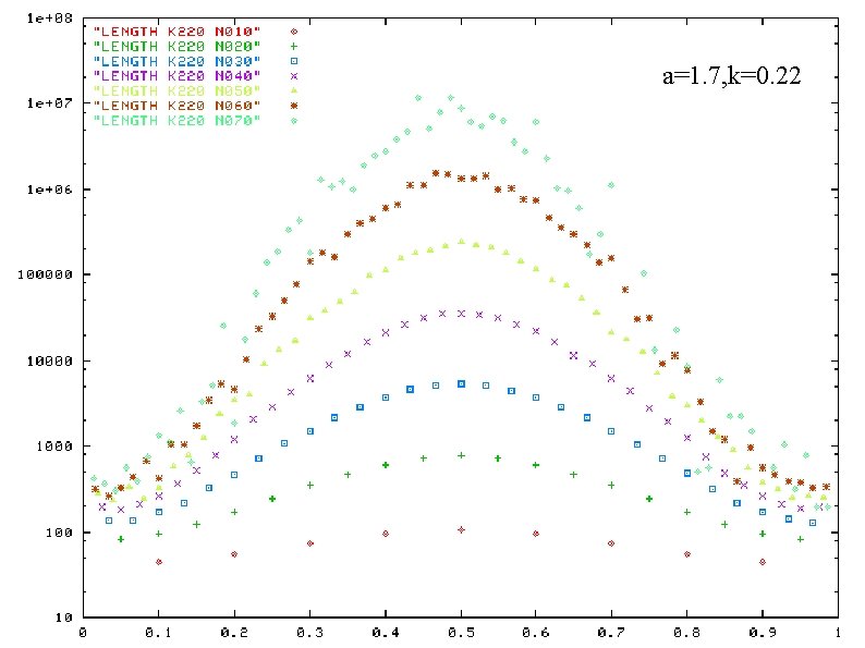
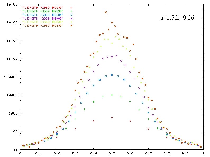
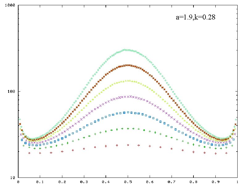
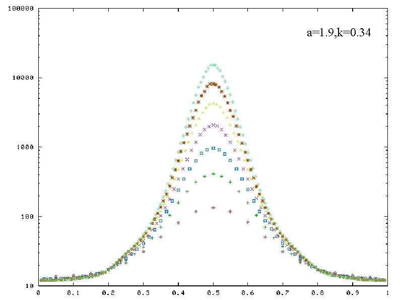
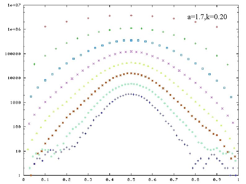
On the mechanism of apparent power-law ● ● ● (1) life-time distribution with fixed a, k and band-weight ratio(w) each of them exhibits clear exponential decay lifetime distribution for fixed a, k, w (2) life-time as a function of band-weight ratio and N (for fixed a, k) smooth dependence on w linear dependence of log(life time) on N Lifetime vs w, N (3) re-injection frequency as a function of band -weight ratio and N (for fixed a, k) smooth dependency on w linear/no dependence of log(life time) on N? Reinjection frequency (2) and (3) leads to emergence of the power-law range in life-time distribution width of the power-law range (in log-scale) that grows linearly with N

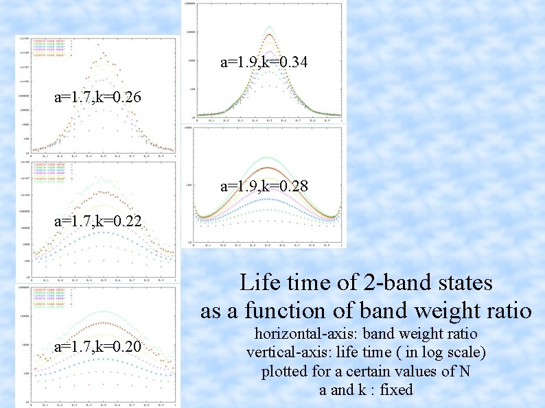
a=1. 9, k=0. 34 a=1. 7, k=0. 26 a=1. 9, k=0. 28 a=1. 7, k=0. 22 Life time of 2 -band states as a function of band weight ratio a=1. 7, k=0. 20 horizontal-axis: band weight ratio vertical-axis: life time ( in log scale) plotted for a certain values of N a and k : fixed

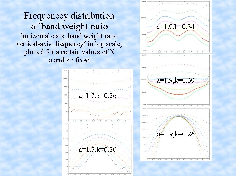
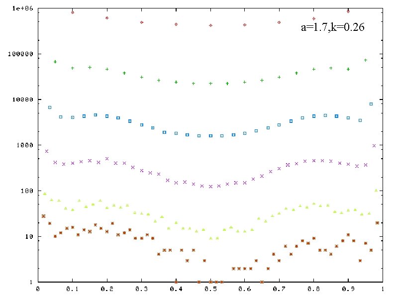
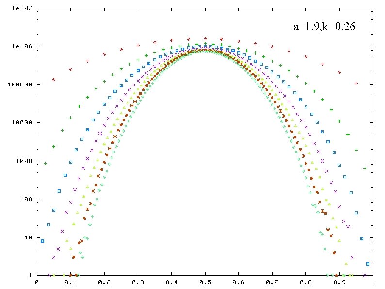
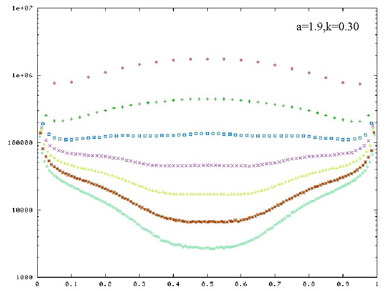
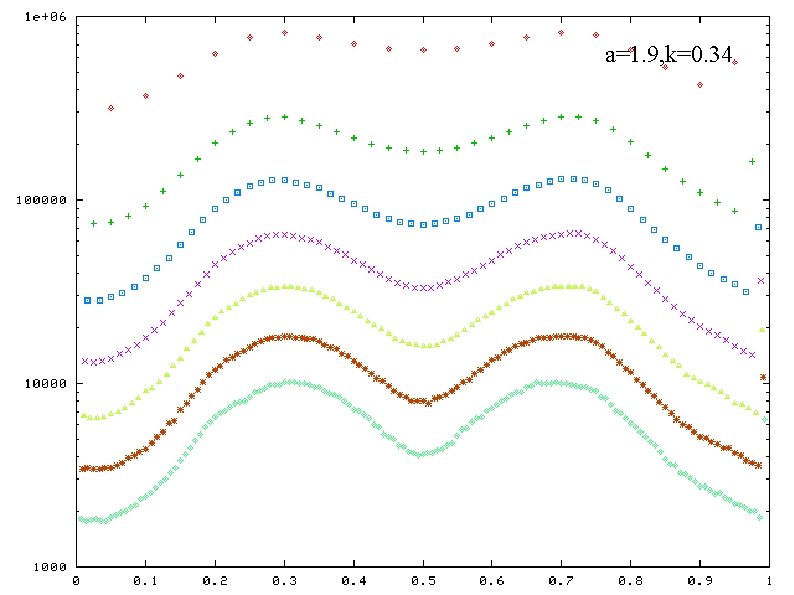
Frequencey distribution of band weight ratio a=1. 9, k=0. 34 horizontal-axis: band weight ratio vertical-axis: frequency( in log scale) plotted for a certain values of N a and k : fixed a=1. 9, k=0. 30 a=1. 7, k=0. 26 a=1. 9, k=0. 26 a=1. 7, k=0. 20

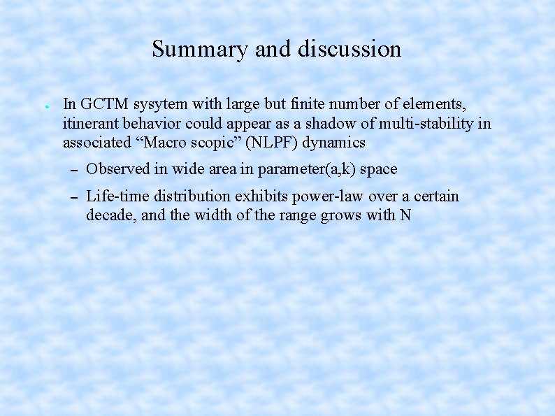
Summary and discussion ● In GCTM sysytem with large but finite number of elements, itinerant behavior could appear as a shadow of multi-stability in associated “Macro scopic” (NLPF) dynamics – Observed in wide area in parameter(a, k) space – Life-time distribution exhibits power-law over a certain decade, and the width of the range grows with N

a=1. 7, k=0. 20

a=1. 7, k=0. 22

a=1. 7, k=0. 26

a=1. 9, k=0. 28

a=1. 9, k=0. 34

a=1. 7, k=0. 20

a=1. 7, k=0. 26

a=1. 9, k=0. 26

a=1. 9, k=0. 30

a=1. 9, k=0. 34