Logistic Regression in jupyter 2017 11 02 Packages

Logistic Regression in jupyter 2017. 11. 02 이완곤 숭실대학교

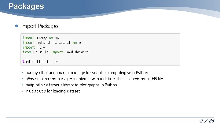
Packages Import Packages • • numpy : the fundamental package for scientific computing with Python h 5 py : a common package to interact with a dataset that is stored on an H 5 file matplotlib : a famous library to plot graphs in Python lr_utils : utils for loading dataset 2 / 25

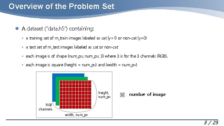
Overview of the Problem Set A dataset (“data. h 5”) containing: • a training set of m_train images labeled as cat (y=1) or non-cat (y=0) • a test set of m_test images labeled as cat or non-cat • each image is of shape (num_px, 3) where 3 is for the 3 channels (RGB). • each image is square (height = num_px) and (width = num_px) height, num_px number of image RGB channels width, num_px 3 / 25

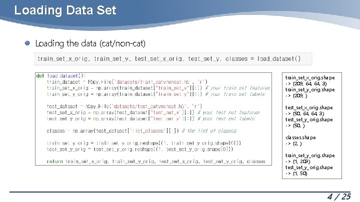
Loading Data Set Loading the data (cat/non-cat) train_set_x_orig. shape -> (209, 64, 3) train_set_y_orig. shape -> (209, ) test_set_x_orig. shape -> (50, 64, 3) test_set_y_orig. shape -> (50, ) classes. shape -> (2, ) train_set_y_orig. shape -> (1, 209) test_set_y_orig. shape -> (1, 50) 4 / 25

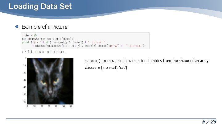
Loading Data Set Example of a Picture squeeze() : remove single-dimensional entries from the shape of an array classes = [‘non-cat’, ‘cat’] 5 / 25

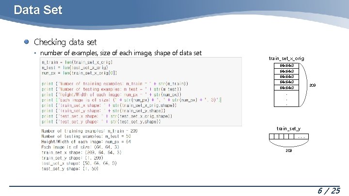
Data Set Checking data set • number of examples, size of each image, shape of data set train_set_x_orig 64 x 64 x 3 64 x 3 209 . . . train_set_y. . . 209 6 / 25

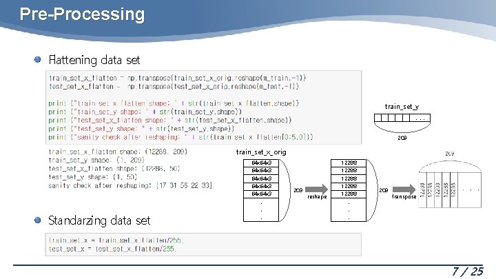
Pre-Processing Flattening data set train_set_y. . . 209 train_set_x_orig 64 x 64 x 3 64 x 3 Standarzing data set . . . 209 reshape 12288 12288 . . . 209 transpose 7 / 25

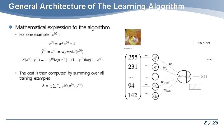
General Architecture of The Learning Algorithm 8 / 25

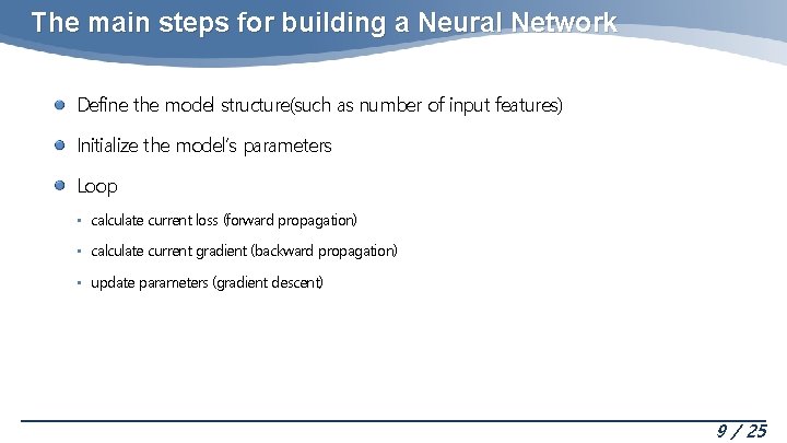
The main steps for building a Neural Network Define the model structure(such as number of input features) Initialize the model’s parameters Loop • calculate current loss (forward propagation) • calculate current gradient (backward propagation) • update parameters (gradient descent) 9 / 25

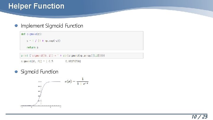
Helper Function Implement Sigmoid Function 10 / 25

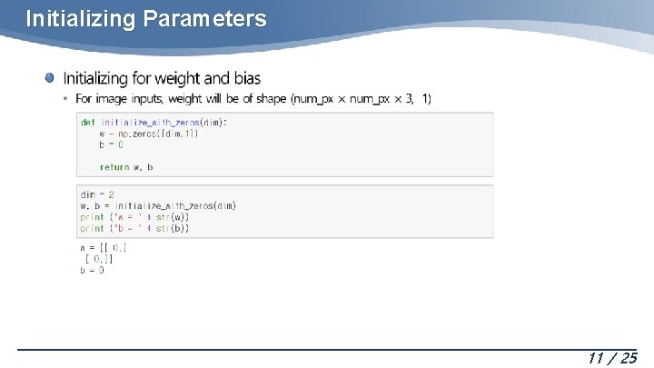
Initializing Parameters 11 / 25

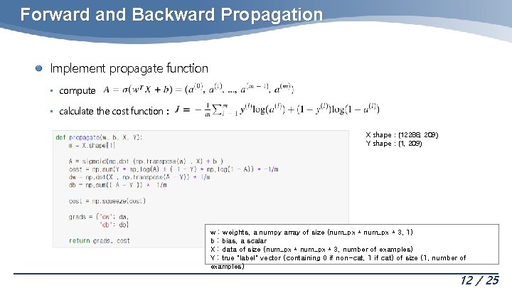
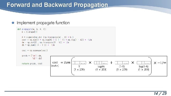
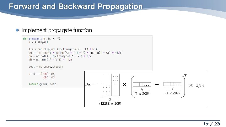
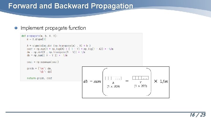
Forward and Backward Propagation Implement propagate function • compute • calculate the cost function : X shape : (12288, 209) Y shape : (1, 209) w : weights, a numpy array of size (num_px * 3, 1) b : bias, a scalar X : data of size (num_px * 3, number of examples) Y : true "label" vector (containing 0 if non-cat, 1 if cat) of size (1, number of examples) 12 / 25

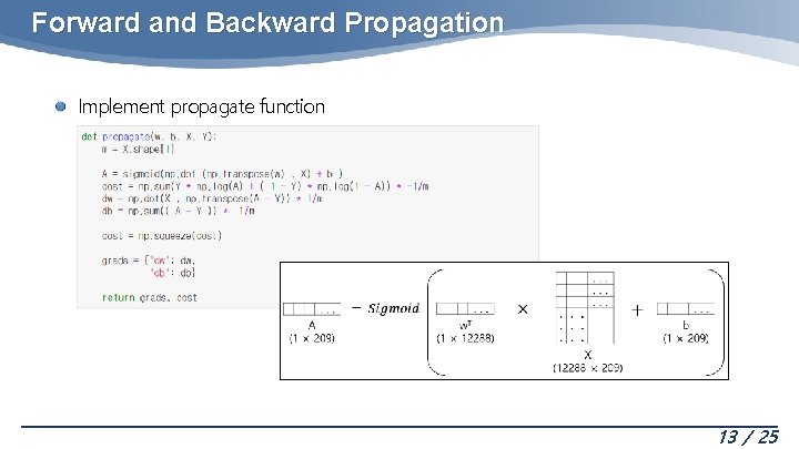
Forward and Backward Propagation Implement propagate function 13 / 25

Forward and Backward Propagation Implement propagate function 14 / 25

Forward and Backward Propagation Implement propagate function 15 / 25

Forward and Backward Propagation Implement propagate function 16 / 25

Parameter Optimizing = … … … [12288 x 1 ] = [scalar] 17 / 25

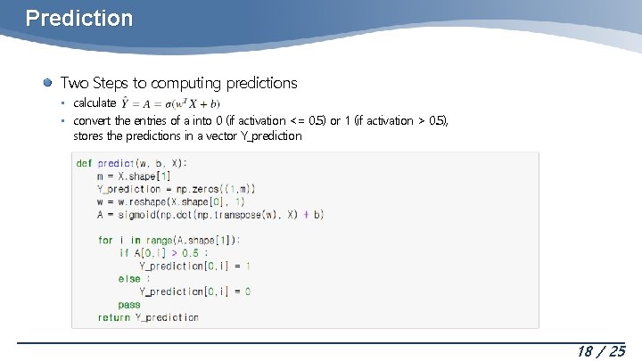
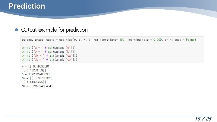
Prediction Two Steps to computing predictions • calculate • convert the entries of a into 0 (if activation <= 0. 5) or 1 (if activation > 0. 5), stores the predictions in a vector Y_prediction 18 / 25

Prediction Output example for prediction 19 / 25

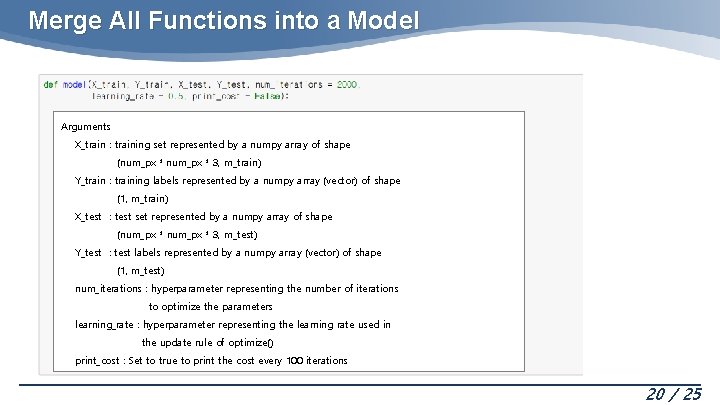
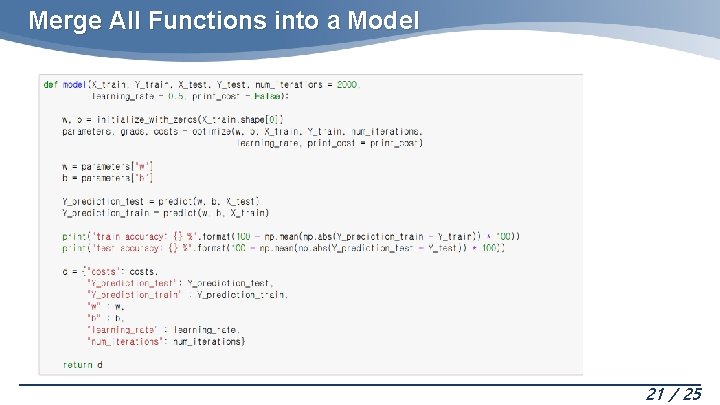
Merge All Functions into a Model Arguments X_train : training set represented by a numpy array of shape (num_px * 3, m_train) Y_train : training labels represented by a numpy array (vector) of shape (1, m_train) X_test : test set represented by a numpy array of shape (num_px * 3, m_test) Y_test : test labels represented by a numpy array (vector) of shape (1, m_test) num_iterations : hyperparameter representing the number of iterations to optimize the parameters learning_rate : hyperparameter representing the learning rate used in the update rule of optimize() print_cost : Set to true to print the cost every 100 iterations 20 / 25

Merge All Functions into a Model 21 / 25

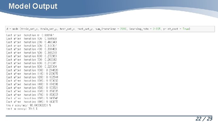
Model Output 22 / 25

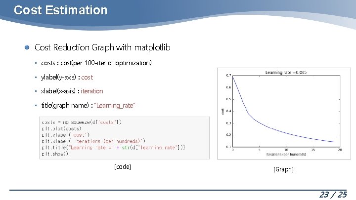
Cost Estimation Cost Reduction Graph with matplotlib • costs : cost(per 100 -iter of optimization) • ylabel(y-axis) : cost • xlabel(x-axis) : iteration • title(graph name) : “Learning_rate” [code] [Graph] 23 / 25

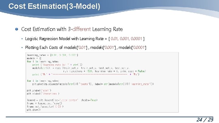
Cost Estimation(3 -Model) Cost Estimation with 3 -different Learning Rate • Logistic Regression Model with Learning Rate = [ 0. 01, 0. 0001 ] • Plotting Each Costs of models[‘ 0. 01’] , models[‘ 0. 0001’] 24 / 25

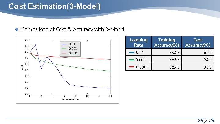
Cost Estimation(3 -Model) Comparison of Cost & Accuracy with 3 -Model Learning Rate Training Accuracy(%) Test Accuracy(%) 0. 01 99. 52 68. 0 0. 001 88. 96 64. 0 0. 0001 68. 42 36. 0 25 / 25