Logistic Regression III SIT 095 The Collection and

Logistic Regression III SIT 095 The Collection and Analysis of Quantitative Data II Week 9 Luke Sloan

Introduction • Recap – Last Week • Workshop Feedback • Multinomial Logistic Regression in SPSS • Model Interpretation • In Class Exercise • Writing-Up • Summary

Recap – Last Week • Variable selection • Binary logistic regression in SPSS • Model interpretation • Intuitive results?

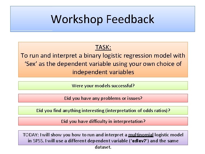
Workshop Feedback TASK: To run and interpret a binary logistic regression model with ‘Sex’ as the dependent variable using your own choice of independent variables Were your models successful? Did you have any problems or issues? Did you find anything interesting (interpretation of odds ratios)? Did you have difficulty in interpretation? TODAY: I will show you how to run and interpret a multinomial logistic model in SPSS. I will use a different dependent variable (‘edlev 7’) and the same dataset.

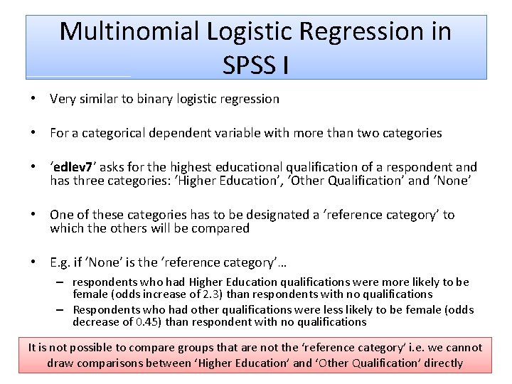
Multinomial Logistic Regression in SPSS I • Very similar to binary logistic regression • For a categorical dependent variable with more than two categories • ‘edlev 7’ asks for the highest educational qualification of a respondent and has three categories: ‘Higher Education’, ‘Other Qualification’ and ‘None’ • One of these categories has to be designated a ‘reference category’ to which the others will be compared • E. g. if ‘None’ is the ‘reference category’… – respondents who had Higher Education qualifications were more likely to be female (odds increase of 2. 3) than respondents with no qualifications – Respondents who had other qualifications were less likely to be female (odds decrease of 0. 45) than respondent with no qualifications It is not possible to compare groups that are not the ‘reference category’ i. e. we cannot draw comparisons between ‘Higher Education’ and ‘Other Qualification’ directly

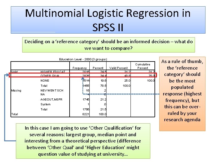
Multinomial Logistic Regression in SPSS II Deciding on a ‘reference category’ should be an informed decision – what do we want to compare? Education Level - 2000 (3 groups) Frequency 2015 2826 Percent 24. 5 34. 4 Valid Percent 31. 2 43. 8 Cumulative Percent 31. 2 75. 0 NONE 1614 19. 6 25. 0 100. 0 Total 6455 78. 5 100. 0 NEV WENT SCH NA 16 4 . 2. 0 AGEOUT, MSPR 1745 21. 2 1 . 0 1766 21. 5 8221 100. 0 Valid Missing HIGHER EDUCAT OTHER QUAL System Total In this case I am going to use ‘Other Qualification’ for several reasons: largest group, median point and interesting from a theoretical perspective (difference between ‘Other Qual’ and ‘Higher Education’ might question value of studying at university… As a rule of thumb, the ‘reference category’ should be the most populated response (highest frequency), but this can be overruled by your research agenda

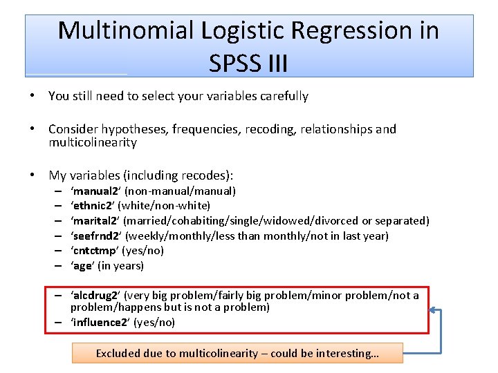
Multinomial Logistic Regression in SPSS III • You still need to select your variables carefully • Consider hypotheses, frequencies, recoding, relationships and multicolinearity • My variables (including recodes): – – – ‘manual 2’ (non-manual/manual) ‘ethnic 2’ (white/non-white) ‘marital 2’ (married/cohabiting/single/widowed/divorced or separated) ‘seefrnd 2’ (weekly/monthly/less than monthly/not in last year) ‘cntctmp’ (yes/no) ‘age’ (in years) – ‘alcdrug 2’ (very big problem/fairly big problem/minor problem/not a problem/happens but is not a problem) – ‘influence 2’ (yes/no) Excluded due to multicolinearity – could be interesting…

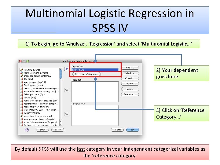
Multinomial Logistic Regression in SPSS IV 1) To begin, go to ‘Analyze’, ‘Regression’ and select ‘Multinomial Logistic…’ 2) Your dependent goes here 3) Click on ‘Reference Category…’ By default SPSS will use the last category in your independent categorical variables as the ‘reference category’

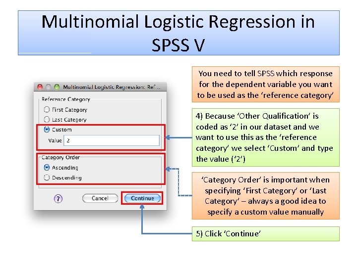
Multinomial Logistic Regression in SPSS V You need to tell SPSS which response for the dependent variable you want to be used as the ‘reference category’ 4) Because ‘Other Qualification’ is coded as ‘ 2’ in our dataset and we want to use this as the ‘reference category’ we select ‘Custom’ and type the value (‘ 2’) ‘Category Order’ is important when specifying ‘First Category’ or ‘Last Category’ – always a good idea to specify a custom value manually 5) Click ‘Continue’

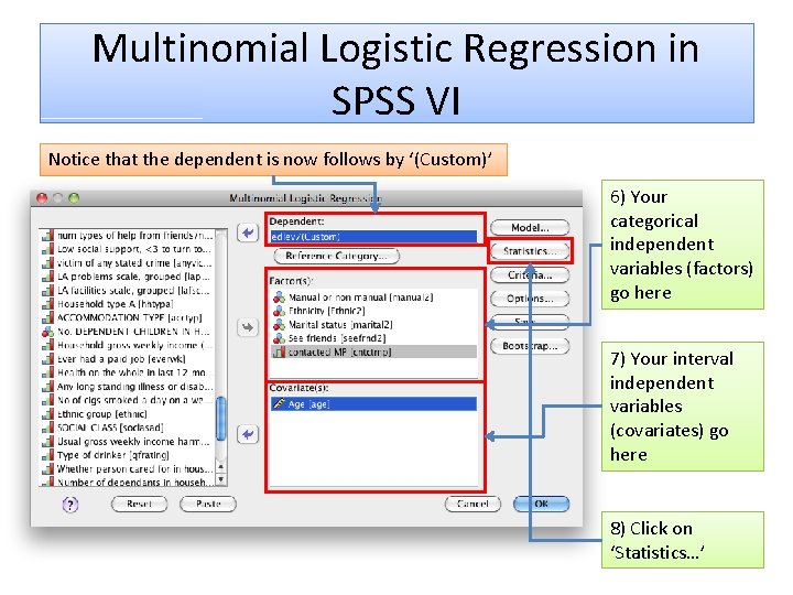
Multinomial Logistic Regression in SPSS VI Notice that the dependent is now follows by ‘(Custom)’ 6) Your categorical independent variables (factors) go here 7) Your interval independent variables (covariates) go here 8) Click on ‘Statistics…’

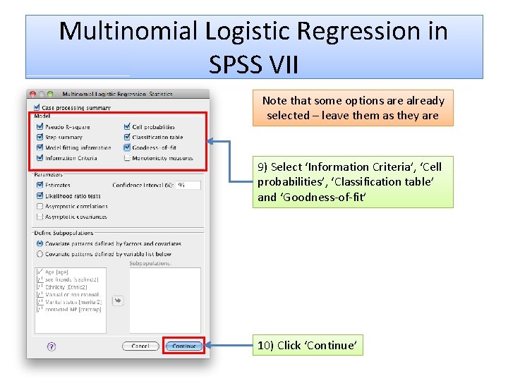
Multinomial Logistic Regression in SPSS VII Note that some options are already selected – leave them as they are 9) Select ‘Information Criteria’, ‘Cell probabilities’, ‘Classification table’ and ‘Goodness-of-fit’ 10) Click ‘Continue’

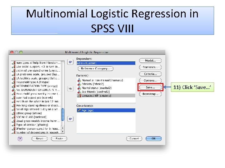
Multinomial Logistic Regression in SPSS VIII 11) Click ‘Save…’

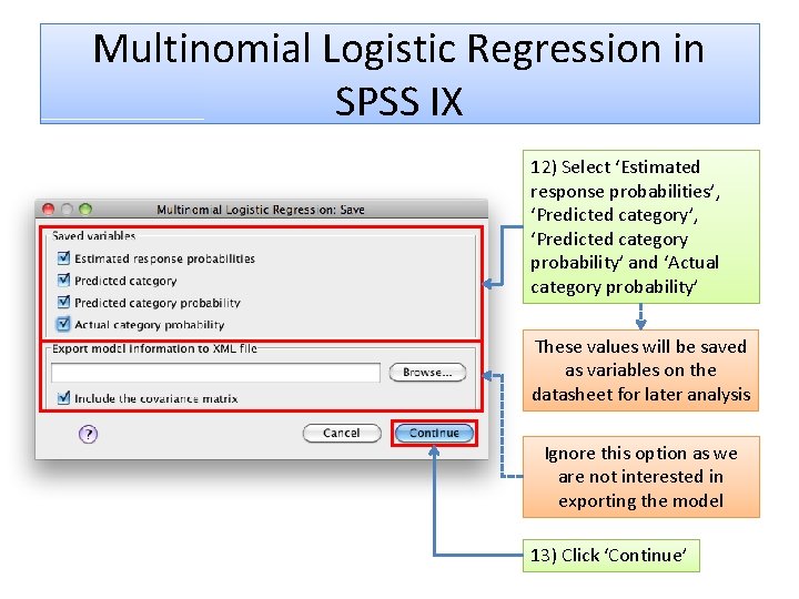
Multinomial Logistic Regression in SPSS IX 12) Select ‘Estimated response probabilities’, ‘Predicted category probability’ and ‘Actual category probability’ These values will be saved as variables on the datasheet for later analysis Ignore this option as we are not interested in exporting the model 13) Click ‘Continue’

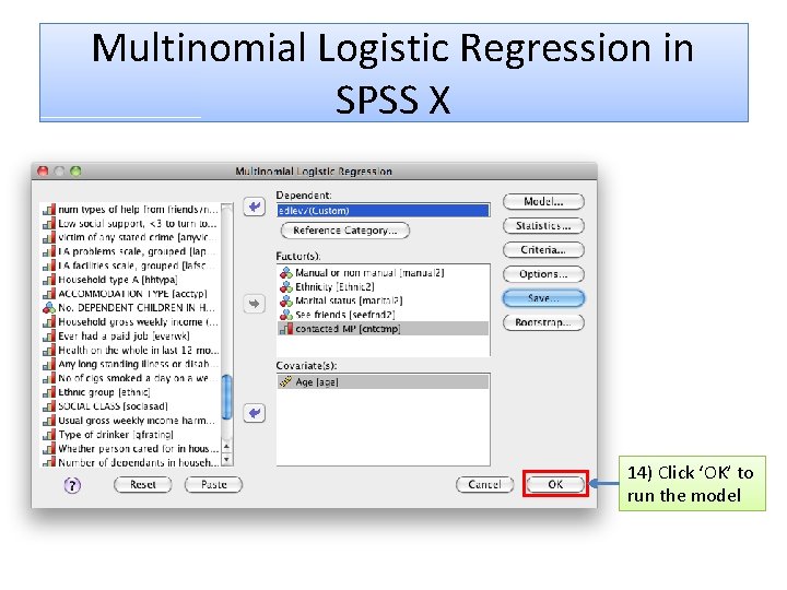
Multinomial Logistic Regression in SPSS X 14) Click ‘OK’ to run the model

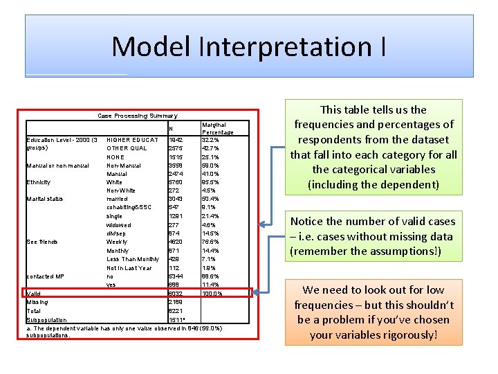
Model Interpretation I Case Processing Summary Marginal Percentage Education Level - 2000 (3 HIGHER EDUCAT 1942 32. 2% groups) OTHER QUAL 2575 42. 7% NONE 1515 25. 1% Manual or non manual Non-Manual 3558 59. 0% Manual 2474 41. 0% Ethnicity White 5760 95. 5% Non-White 272 4. 5% Marital status married 3043 50. 4% cohabiting&SSC 547 9. 1% single 1291 21. 4% widowed 277 4. 6% div/sep 874 14. 5% See friends Weekly 4620 76. 6% Monthly 871 14. 4% Less Than Monthly 429 7. 1% Not In Last Year 112 1. 9% contacted MP no 5344 88. 6% yes 688 11. 4% Valid 6032 100. 0% Missing 2189 Total 8221 a Subpopulation 1511 a. The dependent variable has only one value observed in 846 (56. 0%) subpopulations. N This table tells us the frequencies and percentages of respondents from the dataset that fall into each category for all the categorical variables (including the dependent) Notice the number of valid cases – i. e. cases without missing data (remember the assumptions!) We need to look out for low frequencies – but this shouldn’t be a problem if you’ve chosen your variables rigorously!

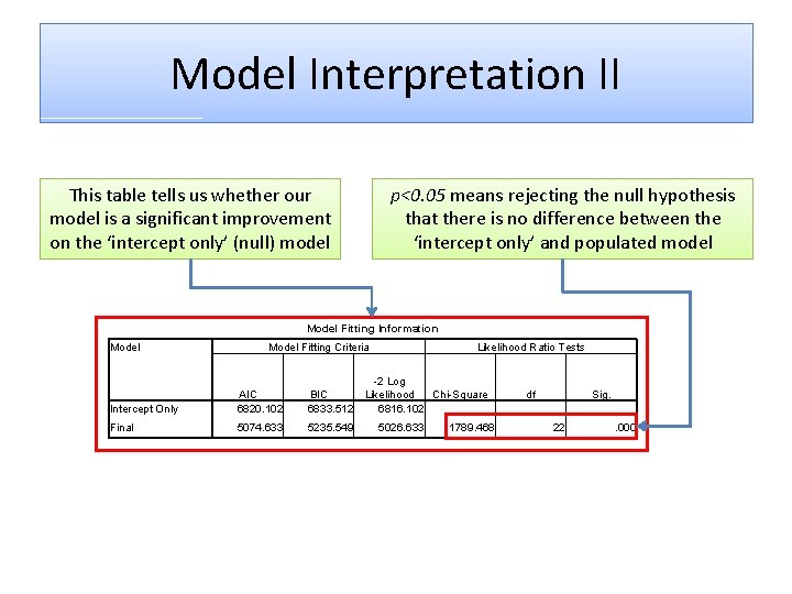
Model Interpretation II This table tells us whether our model is a significant improvement on the ‘intercept only’ (null) model p<0. 05 means rejecting the null hypothesis that there is no difference between the ‘intercept only’ and populated model Model Fitting Information Model Fitting Criteria Intercept Only AIC 6820. 102 BIC 6833. 512 Final 5074. 633 5235. 549 Likelihood Ratio Tests -2 Log Likelihood Chi-Square 6816. 102 5026. 633 1789. 468 df Sig. 22 . 000

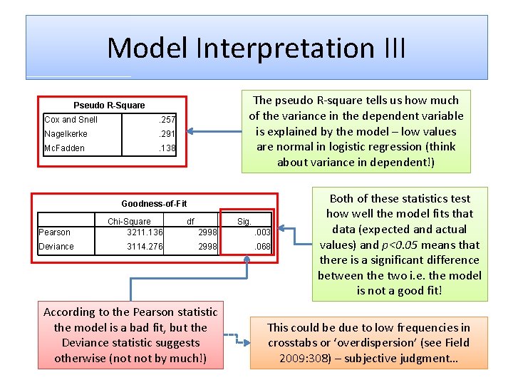
Model Interpretation III The pseudo R-square tells us how much of the variance in the dependent variable is explained by the model – low values are normal in logistic regression (think about variance in dependent!) Pseudo R-Square Cox and Snell . 257 Nagelkerke . 291 Mc. Fadden . 138 Goodness-of-Fit Pearson Deviance Chi-Square 3211. 136 3114. 276 df Sig. 2998 . 003 2998 . 068 According to the Pearson statistic the model is a bad fit, but the Deviance statistic suggests otherwise (not by much!) Both of these statistics test how well the model fits that data (expected and actual values) and p<0. 05 means that there is a significant difference between the two i. e. the model is not a good fit! This could be due to low frequencies in crosstabs or ‘overdispersion’ (see Field 2009: 308) – subjective judgment…

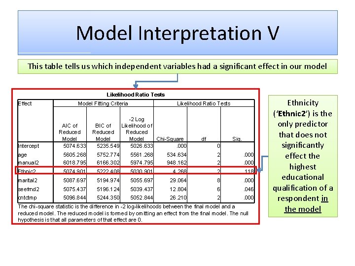
Model Interpretation V This table tells us which independent variables had a significant effect in our model Likelihood Ratio Tests Effect Model Fitting Criteria Likelihood Ratio Tests -2 Log BIC of Likelihood of Reduced Model Chi-Square 5235. 549 5026. 633. 000 Intercept AIC of Reduced Model 5074. 633 age manual 2 5605. 268 6018. 795 5752. 774 6166. 302 5561. 268 5974. 795 Ethnic 2 5074. 901 5222. 408 marital 2 5087. 697 seefrnd 2 cntctmp df Sig. 0 . 534. 634 948. 162 2 2 . 000 5030. 901 4. 268 2 . 118 5194. 974 5055. 697 29. 064 8 . 000 5075. 437 5196. 124 5039. 437 12. 804 6 . 046 5096. 844 5244. 350 5052. 844 26. 210 2 . 000 The chi-square statistic is the difference in -2 log-likelihoods between the final model and a reduced model. The reduced model is formed by omitting an effect from the final model. The null hypothesis is that all parameters of that effect are 0. Ethnicity (‘Ethnic 2’) is the only predictor that does not significantly effect the highest educational qualification of a respondent in the model

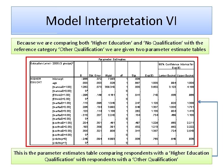
Model Interpretation VI Because we are comparing both ‘Higher Education’ and ‘No Qualification’ with the reference category ‘Other Qualification’ we are given two parameter estimate tables Parameter Estimates Education Level - 2000 (3 groups)a HIGHER EDUCAT Intercept age [manual 2=1. 00] [manual 2=2. 00] [Ethnic 2=1. 00] [Ethnic 2=2. 00] [marital 2=1. 00] [marital 2=2. 00] [marital 2=3. 00] [marital 2=4. 00] [marital 2=5. 00] [seefrnd 2=1. 00] [seefrnd 2=2. 00] [seefrnd 2=3. 00] [seefrnd 2=4. 00] [cntctmp=1] 95% Confidence Interval for Exp(B) B Std. Error Wald -. 988. 372 7. 063. 000. 003. 028 1. 282. 073 309. 342 0 b. . -. 298. 146 4. 181 0 b. . . 113. 098 1. 340. 268. 134 3. 992. 123. 114 1. 156 -. 310. 207 2. 242 0 b. . . 204. 301. 461. 193. 309. 391. 305. 321. 906 0 b. . -. 249. 094 6. 993 0 b. . df 1 1 1 0 1 1 1 0 Sig. . 008. 867. 000. . 041. . 247. 046. 282. 134. . 497. 532. 341. . 008. Exp(B) Lower Bound Upper Bound 1. 000. 994 1. 005 3. 602 3. 123 4. 156. . 742. 558. 988. . . 1. 120. 925 1. 356 1. 307 1. 005 1. 701 1. 130. 904 1. 413. 734. 489 1. 100. . . 1. 226. 680 2. 211 1. 213. 662 2. 222 1. 357. 724 2. 543. . 780. 649. 938. . . This is the parameter estimates table comparing respondents with a ‘Higher Education Qualification’ with respondents with a ‘Other Qualification’

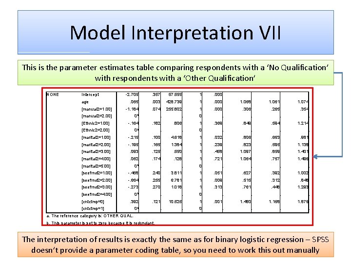
Model Interpretation VII This is the parameter estimates table comparing respondents with a ‘No Qualification’ with respondents with a ‘Other Qualification’ NONE Intercept -2. 705 . 357 57. 555 1 . 000 . 065 . 003 428. 739 1 . 000 1. 068 1. 061 1. 074 [manual 2=1. 00] -1. 184 . 074 255. 802 1 . 000 . 306 . 265 . 354 [manual 2=2. 00] 0 b . . 0 . . [Ethnic 2=1. 00] -. 164 . 182 . 806 1 . 369 . 849 . 594 1. 214 [Ethnic 2=2. 00] 0 b . . 0 . . [marital 2=1. 00] -. 215 . 100 4. 618 1 . 032 . 806 . 663 . 981 [marital 2=2. 00] -. 195 . 165 1. 384 1 . 239 . 823 . 595 1. 138 [marital 2=3. 00] . 093 . 125 . 550 1 . 458 1. 097 . 859 1. 401 [marital 2=4. 00] . 062 . 174 . 128 1 . 721 1. 064 . 757 1. 496 [marital 2=5. 00] 0 b . . 0 . . [seefrnd 2=1. 00] -. 468 . 240 3. 811 1 . 051 . 627 . 392 1. 002 [seefrnd 2=2. 00] -. 664 . 255 6. 781 1 . 009 . 515 . 312 . 848 [seefrnd 2=3. 00] -. 273 . 270 1. 018 1 . 313 . 761 . 448 1. 293 [seefrnd 2=4. 00] 0 b . . 0 . . [cntctmp=0] . 392 . 121 10. 525 1 . 001 1. 480 1. 168 1. 875 [cntctmp=1] 0 b . . 0 . . age a. The reference category is: OTHER QUAL. b. This parameter is set to zero because it is redundant. The interpretation of results is exactly the same as for binary logistic regression – SPSS doesn’t provide a parameter coding table, so you need to work this out manually

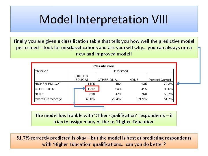
Model Interpretation VIII Finally you are given a classification table that tells you how well the predictive model performed – look for misclassifications and ask yourself why… you can always run a new and improved model! Classification Observed HIGHER EDUCAT OTHER QUAL NONE Overall Percentage Predicted HIGHER EDUCAT OTHER QUAL 1405 402 NONE 135 Percent Correct 72. 3% 1217 943 415 36. 6% 319 428 768 50. 7% 48. 8% 29. 4% 21. 9% 51. 7% The model has trouble with ‘Other Qualification’ respondents – it tries to assign many of the to ‘Higher Education’ 51. 7% correctly predicted is okay – but the model is best at predicting respondents with ‘Higher Education’ qualifications… can you do better?

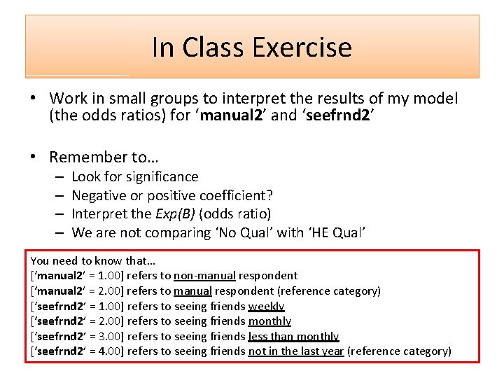
In Class Exercise • Work in small groups to interpret the results of my model (the odds ratios) for ‘manual 2’ and ‘seefrnd 2’ • Remember to… – – Look for significance Negative or positive coefficient? Interpret the Exp(B) (odds ratio) We are not comparing ‘No Qual’ with ‘HE Qual’ You need to know that… [‘manual 2’ = 1. 00] refers to non-manual respondent [‘manual 2’ = 2. 00] refers to manual respondent (reference category) [‘seefrnd 2’ = 1. 00] refers to seeing friends weekly [‘seefrnd 2’ = 2. 00] refers to seeing friends monthly [‘seefrnd 2’ = 3. 00] refers to seeing friends less than monthly [‘seefrnd 2’ = 4. 00] refers to seeing friends not in the last year (reference category)

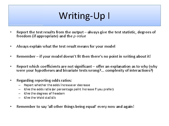
Writing-Up I • Report the test results from the output – always give the test statistic, degrees of freedom (if appropriate) and the p-value • Always explain what the test result means for your model • Remember – if your model doesn’t fit then there’s no point in writing about it! • Report which coefficients are not significant – offer an explanation as to why (why were your hypotheses and bivariate tests wrong? . . . complexity of interactions? ) • Regarding reporting odds ratios: – – • Report whether the odds increase or decrease Give the odds ratio (or percentage point increase if you prefer) Give the degrees of freedom Give the Wald statistic Remember to say ‘all other things being equal’ every now and again!

Writing-Up II EXAMPLE: The coefficient for the variable ‘manual 2’ (whether a respondent has a manual or nonmanual occupation) was significant for both respondents with a higher education and no qualification. Non-manual respondents were much more likely to have a higher education than an ‘other’ qualification than manual respondents (odds = 3. 6, 1 d. f. , Wald = 309. 34) all other things being equal. Also, non-manual respondents were much less likely not to have any qualifications than to have an ‘other’ qualification than manual respondents (odds = 0. 31, 1 d. f. , Wald = 255. 80) all other things being equal. Although the language is awkward we can summarise by saying that respondents with higher education qualifications are more likely to have non-manual jobs than respondents with ‘other’ qualifications. Also, respondents with no qualifications are less likely to have non-manual jobs than respondents with ‘other’ qualifications. Both of these statements are made in reference to respondents who have manual occupations (the dummy ref cat. ) and with ‘other’ qualifications (DV ref cat. )

Summary • Binary and multinomial models are very similar, but notice the subtle differences • Again interpretation of the coefficients and Exp(B) are the tricky bit • The models are very powerful, even when saying ‘more likely’ or ‘less likely’

Workshop Task • Run a multinomial logistic regression model with the dependent variable ‘edlev 7’ • See if you can get a better prediction rate than me! • Use everything you’ve learnt over the past weeks, starting with the proper procedure for variable selection • Use these slides to check that the model works (follow my step-by-step guide to operation and interpretation) • Interpret the odds ratios and draw some conclusions about your model • If your model doesn’t work then work in pairs • This technique is advanced, so ask for help if you are unsure