Logistic Regression EPP 245298 Statistical Analysis of Laboratory

Logistic Regression EPP 245/298 Statistical Analysis of Laboratory Data 1

Generalized Linear Models • The type of predictive model one uses depends on a number of issues; one is the type of response. • Measured values such as quantity of a protein, age, weight usually can be handled in an ordinary linear regression model • Patient survival, which may be censored, calls for a different method (next quarter) November 10, 2004 EPP 245 Statistical Analysis of Laboratory Data 2

• If the response is binary, then can we use logistic regression models • If the response is a count, we can use Poisson regression • Other forms of response can generate other types of generalized linear models November 10, 2004 EPP 245 Statistical Analysis of Laboratory Data 3

Generalized Linear Models • We need a linear predictor of the same form as in linear regression βx • In theory, such a linear predictor can generate any type of number as a prediction, positive, negative, or zero • We choose a suitable distribution for the type of data we are predicting (normal for any number, gamma for positive numbers, binomial for binary responses, Poisson for counts) • We create a link function which maps the mean of the distribution onto the set of all possible linear prediction results, which is the whole real line (-∞, ∞). • The inverse of the link function takes the linear predictor to the actual prediction November 10, 2004 EPP 245 Statistical Analysis of Laboratory Data 4

• Ordinary linear regression has identity link (no transformation by the link function) and uses the normal distribution • If one is predicting an inherently positive quantity, one may want to use the log link since ex is always positive. • An alternative to using a generalized linear model with an log link, is to transform the data using the log or maybe glog. This is a device that works well with measurement data but may not be usable in other cases November 10, 2004 EPP 245 Statistical Analysis of Laboratory Data 5

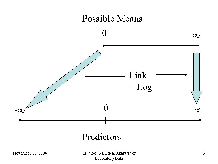
Possible Means 0 ∞ Link = Log -∞ 0 ∞ Predictors November 10, 2004 EPP 245 Statistical Analysis of Laboratory Data 6

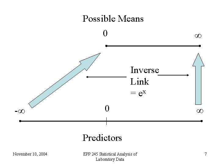
Possible Means 0 ∞ Inverse Link = ex -∞ 0 ∞ Predictors November 10, 2004 EPP 245 Statistical Analysis of Laboratory Data 7

Logistic Regression • Suppose we are trying to predict a binary variable (patient has ovarian cancer or not, patient is responding to therapy or not) • We can describe this by a 0/1 variable in which the value 1 is used for one response (patient has ovarian cancer) and 0 for the other (patient does not have ovarian cancer • We can then try to predict this response November 10, 2004 EPP 245 Statistical Analysis of Laboratory Data 8

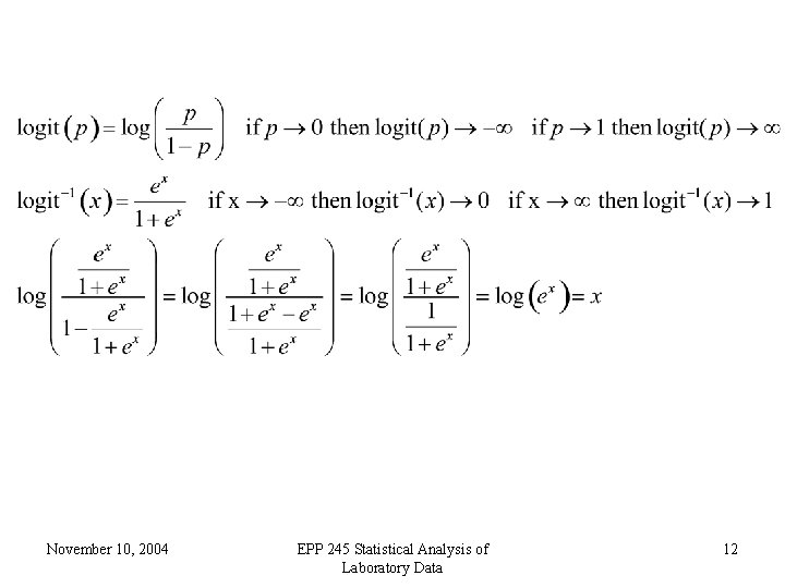
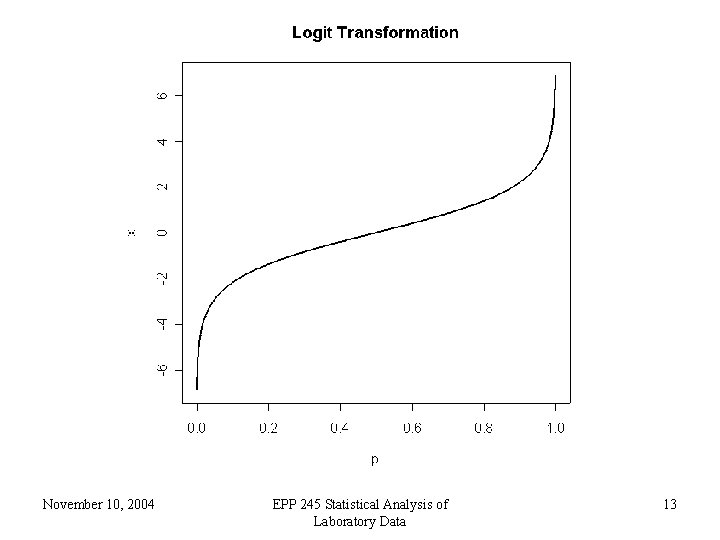
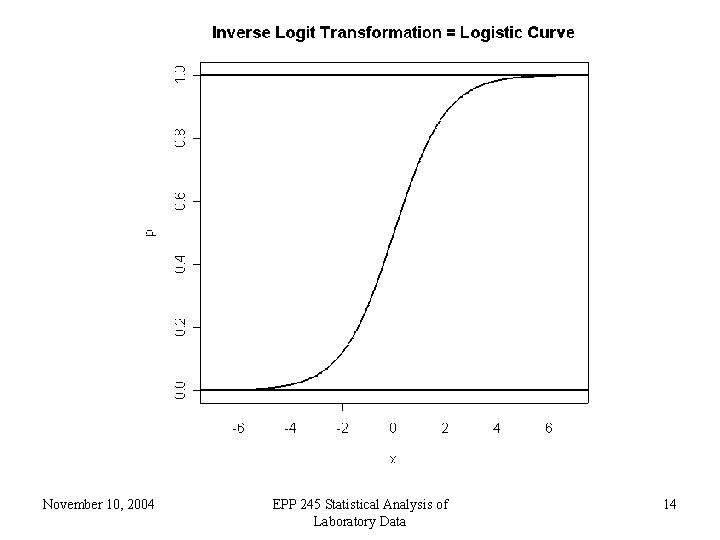
• For a given patient, a prediction can be thought of as a kind of probability that the patient does have ovarian cancer. As such, the prediction should be between 0 and 1. Thus ordinary linear regression is not suitable • The logit transform takes a number which can be anything, positive or negative, and produces a number between 0 and 1. Thus the logit link is useful for binary data November 10, 2004 EPP 245 Statistical Analysis of Laboratory Data 9

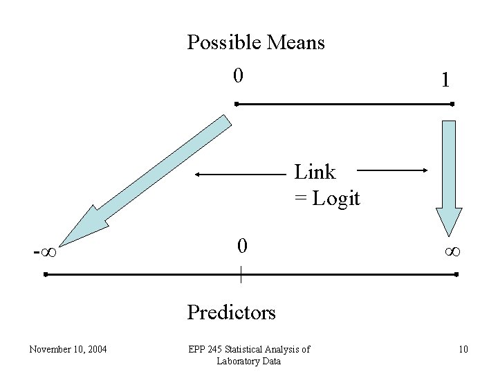
Possible Means 0 1 Link = Logit -∞ 0 ∞ Predictors November 10, 2004 EPP 245 Statistical Analysis of Laboratory Data 10

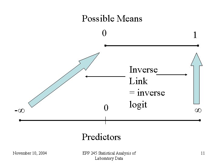
Possible Means 0 -∞ 0 Inverse Link = inverse logit 1 ∞ Predictors November 10, 2004 EPP 245 Statistical Analysis of Laboratory Data 11

November 10, 2004 EPP 245 Statistical Analysis of Laboratory Data 12

November 10, 2004 EPP 245 Statistical Analysis of Laboratory Data 13

November 10, 2004 EPP 245 Statistical Analysis of Laboratory Data 14

Analyzing Tabular Data with Logistic Regression • Example data set from Daalgard p. 193 • Response is hypertensive y/n • Predictors are smoking (y/n), obesity (y/n), snoring (y/n) • How well can these 3 factors explain/predict the presence of hypertension? • Which are important? November 10, 2004 EPP 245 Statistical Analysis of Laboratory Data 15

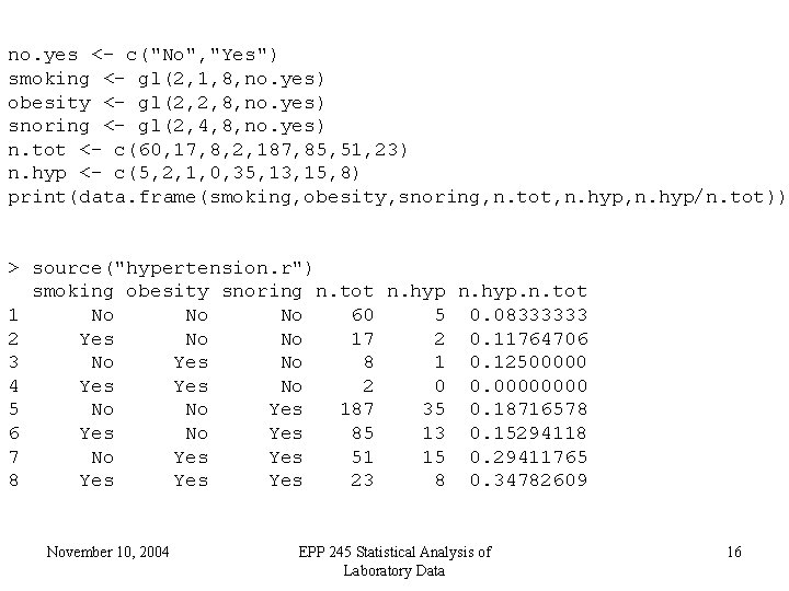
no. yes <- c("No", "Yes") smoking <- gl(2, 1, 8, no. yes) obesity <- gl(2, 2, 8, no. yes) snoring <- gl(2, 4, 8, no. yes) n. tot <- c(60, 17, 8, 2, 187, 85, 51, 23) n. hyp <- c(5, 2, 1, 0, 35, 13, 15, 8) print(data. frame(smoking, obesity, snoring, n. tot, n. hyp/n. tot)) > source("hypertension. r") smoking obesity snoring n. tot n. hyp. n. tot 1 No No No 60 5 0. 08333333 2 Yes No No 17 2 0. 11764706 3 No Yes No 8 1 0. 12500000 4 Yes No 2 0 0. 0000 5 No No Yes 187 35 0. 18716578 6 Yes No Yes 85 13 0. 15294118 7 No Yes 51 15 0. 29411765 8 Yes Yes 23 8 0. 34782609 November 10, 2004 EPP 245 Statistical Analysis of Laboratory Data 16

Specifying Logistic Regressions • For each ‘cell’, we need to specify the diseased and normals, which will be what we try to fit. • This can be specified either as a matrix with one column consisting of the number of diseased persons, and the other the number of normals (not the total). • Or we can specify the proportions as a response, with weights equal to the sample size November 10, 2004 EPP 245 Statistical Analysis of Laboratory Data 17

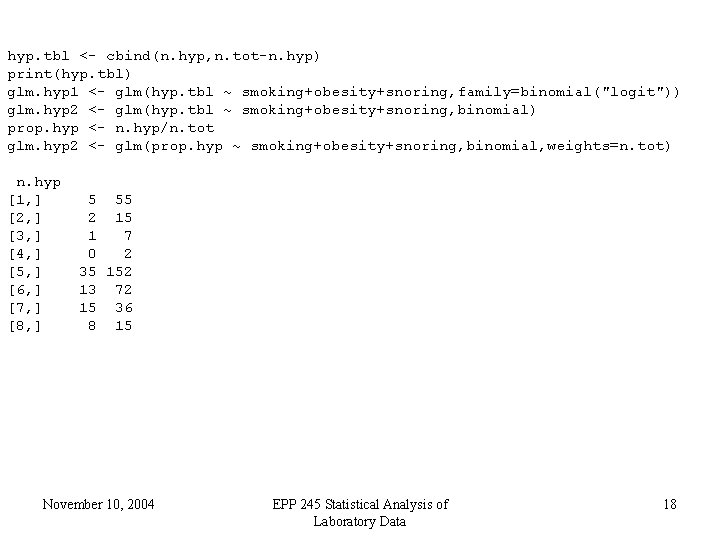
hyp. tbl <- cbind(n. hyp, n. tot-n. hyp) print(hyp. tbl) glm. hyp 1 <- glm(hyp. tbl ~ smoking+obesity+snoring, family=binomial("logit")) glm. hyp 2 <- glm(hyp. tbl ~ smoking+obesity+snoring, binomial) prop. hyp <- n. hyp/n. tot glm. hyp 2 <- glm(prop. hyp ~ smoking+obesity+snoring, binomial, weights=n. tot) n. hyp [1, ] [2, ] [3, ] [4, ] [5, ] [6, ] [7, ] [8, ] 5 55 2 15 1 7 0 2 35 152 13 72 15 36 8 15 November 10, 2004 EPP 245 Statistical Analysis of Laboratory Data 18

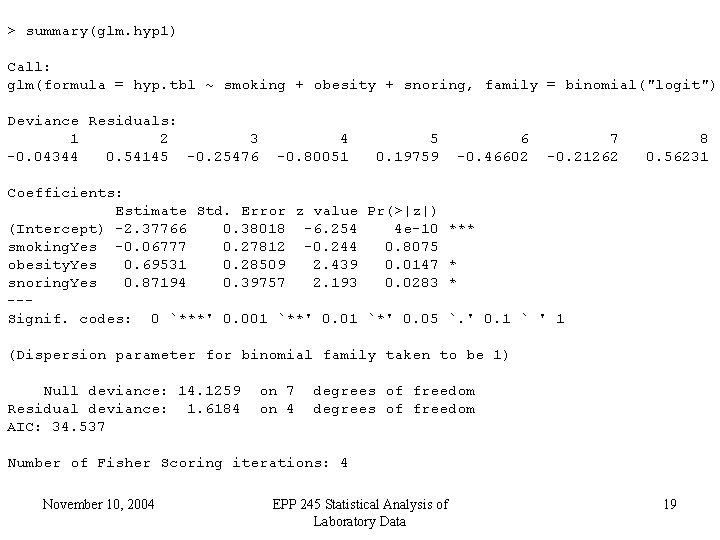
> summary(glm. hyp 1) Call: glm(formula = hyp. tbl ~ smoking + obesity + snoring, family = binomial("logit")) Deviance Residuals: 1 2 3 -0. 04344 0. 54145 -0. 25476 4 -0. 80051 5 0. 19759 6 -0. 46602 7 -0. 21262 8 0. 56231 Coefficients: Estimate Std. Error z value Pr(>|z|) (Intercept) -2. 37766 0. 38018 -6. 254 4 e-10 *** smoking. Yes -0. 06777 0. 27812 -0. 244 0. 8075 obesity. Yes 0. 69531 0. 28509 2. 439 0. 0147 * snoring. Yes 0. 87194 0. 39757 2. 193 0. 0283 * --Signif. codes: 0 `***' 0. 001 `**' 0. 01 `*' 0. 05 `. ' 0. 1 ` ' 1 (Dispersion parameter for binomial family taken to be 1) Null deviance: 14. 1259 Residual deviance: 1. 6184 AIC: 34. 537 on 4 degrees of freedom Number of Fisher Scoring iterations: 4 November 10, 2004 EPP 245 Statistical Analysis of Laboratory Data 19

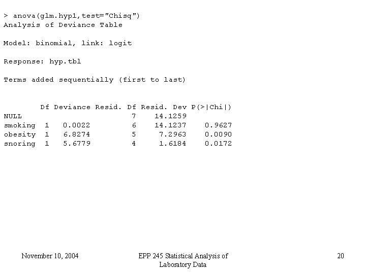
> anova(glm. hyp 1, test="Chisq") Analysis of Deviance Table Model: binomial, link: logit Response: hyp. tbl Terms added sequentially (first to last) Df Deviance Resid. Df Resid. Dev P(>|Chi|) NULL 7 14. 1259 smoking 1 0. 0022 6 14. 1237 0. 9627 obesity 1 6. 8274 5 7. 2963 0. 0090 snoring 1 5. 6779 4 1. 6184 0. 0172 November 10, 2004 EPP 245 Statistical Analysis of Laboratory Data 20

Logistic Regression with Raw Data • Sometimes the data are in the form of individual cases with the covariates and resulting binary classification variable as a 0/1 variable or two-level factor. It is convenient not to have to tabulate • Also, if any of the covariates is continuous, categorization is not possible without discretizing the variable November 10, 2004 EPP 245 Statistical Analysis of Laboratory Data 21

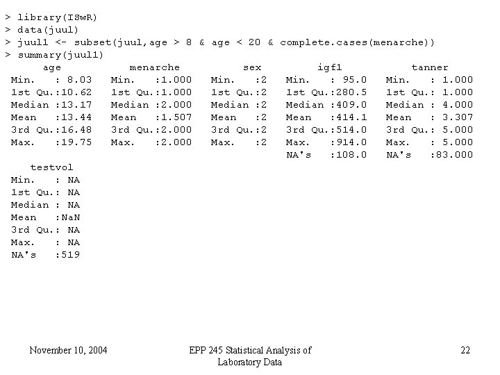
> > library(ISw. R) data(juul) juul 1 <- subset(juul, age > 8 & age < 20 & complete. cases(menarche)) summary(juul 1) age menarche sex igf 1 tanner Min. : 8. 03 Min. : 1. 000 Min. : 2 Min. : 95. 0 Min. : 1. 000 1 st Qu. : 10. 62 1 st Qu. : 1. 000 1 st Qu. : 280. 5 1 st Qu. : 1. 000 Median : 13. 17 Median : 2. 000 Median : 2 Median : 409. 0 Median : 4. 000 Mean : 13. 44 Mean : 1. 507 Mean : 2 Mean : 414. 1 Mean : 3. 307 3 rd Qu. : 16. 48 3 rd Qu. : 2. 000 3 rd Qu. : 2 3 rd Qu. : 514. 0 3 rd Qu. : 5. 000 Max. : 19. 75 Max. : 2. 000 Max. : 2 Max. : 914. 0 Max. : 5. 000 NA's : 108. 0 NA's : 83. 000 testvol Min. : NA 1 st Qu. : NA Median : NA Mean : Na. N 3 rd Qu. : NA Max. : NA NA's : 519 November 10, 2004 EPP 245 Statistical Analysis of Laboratory Data 22

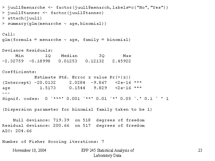
> > juul 1$menarche <- factor(juul 1$menarch, labels=c("No", "Yes")) juul 1$tanner <- factor(juul 1$tanner) attach(juul 1) summary(glm(menarche ~ age, binomial)) Call: glm(formula = menarche ~ age, family = binomial) Deviance Residuals: Min 1 Q -2. 32759 -0. 18998 Median 0. 01253 3 Q 0. 12132 Max 2. 45922 Coefficients: Estimate Std. Error z value Pr(>|z|) (Intercept) -20. 0132 2. 0284 -9. 867 <2 e-16 *** age 1. 5173 0. 1544 9. 829 <2 e-16 *** --Signif. codes: 0 `***' 0. 001 `**' 0. 01 `*' 0. 05 `. ' 0. 1 ` ' 1 (Dispersion parameter for binomial family taken to be 1) Null deviance: 719. 39 Residual deviance: 200. 66 AIC: 204. 66 on 518 on 517 degrees of freedom Number of Fisher Scoring iterations: 7 November 10, 2004 EPP 245 Statistical Analysis of Laboratory Data 23

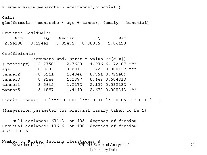
> summary(glm(menarche ~ age+tanner, binomial)) Call: glm(formula = menarche ~ age + tanner, family = binomial) Deviance Residuals: Min 1 Q -2. 56180 -0. 12461 Median 0. 02475 3 Q 0. 08055 Coefficients: Estimate Std. Error z value (Intercept) -13. 7758 2. 7630 -4. 986 age 0. 8603 0. 2311 3. 723 tanner 2 -0. 5211 1. 4846 -0. 351 tanner 3 0. 8264 1. 2377 0. 668 tanner 4 2. 5645 1. 2172 2. 107 tanner 5 5. 1897 1. 4140 3. 670 --Signif. codes: 0 `***' 0. 001 `**' 0. 01 Max 2. 86120 Pr(>|z|) 6. 17 e-07 0. 000197 0. 725609 0. 504313 0. 035132 0. 000242 *** * *** `*' 0. 05 `. ' 0. 1 ` ' 1 (Dispersion parameter for binomial family taken to be 1) Null deviance: 604. 2 Residual deviance: 106. 6 AIC: 118. 6 on 435 on 430 degrees of freedom Number of Fisher Scoring iterations: 8 November 10, 2004 EPP 245 Statistical Analysis of Laboratory Data 24

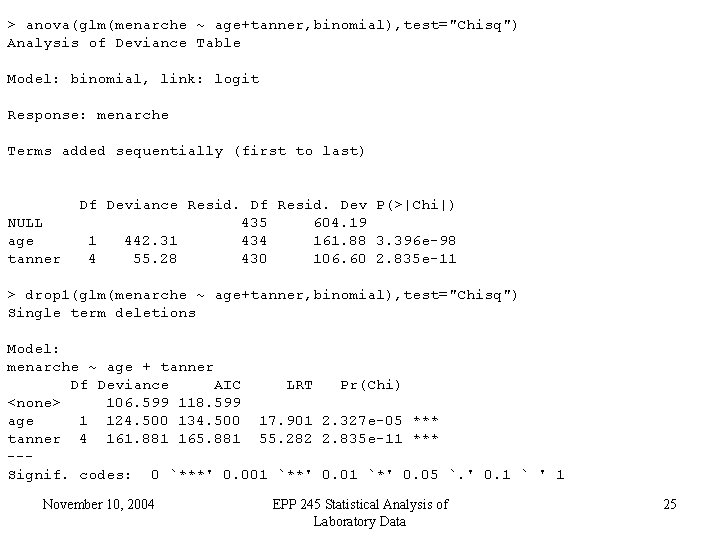
> anova(glm(menarche ~ age+tanner, binomial), test="Chisq") Analysis of Deviance Table Model: binomial, link: logit Response: menarche Terms added sequentially (first to last) NULL age tanner Df Deviance Resid. Df Resid. Dev P(>|Chi|) 435 604. 19 1 442. 31 434 161. 88 3. 396 e-98 4 55. 28 430 106. 60 2. 835 e-11 > drop 1(glm(menarche ~ age+tanner, binomial), test="Chisq") Single term deletions Model: menarche ~ age + tanner Df Deviance AIC LRT Pr(Chi) <none> 106. 599 118. 599 age 1 124. 500 134. 500 17. 901 2. 327 e-05 *** tanner 4 161. 881 165. 881 55. 282 2. 835 e-11 *** --Signif. codes: 0 `***' 0. 001 `**' 0. 01 `*' 0. 05 `. ' 0. 1 ` ' 1 November 10, 2004 EPP 245 Statistical Analysis of Laboratory Data 25

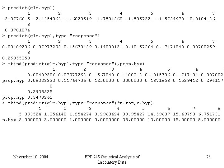
> predict(glm. hyp 1) 1 2 3 4 5 6 7 -2. 3776615 -2. 4454364 -1. 6823519 -1. 7501268 -1. 5057221 -1. 5734970 -0. 8104126 8 -0. 8781874 > predict(glm. hyp 1, type="response") 1 2 3 4 5 6 7 0. 08489206 0. 07977292 0. 15678429 0. 14803121 0. 18157364 0. 17171843 0. 30780259 8 0. 29355353 > rbind(predict(glm. hyp 1, type="response"), prop. hyp) 1 2 3 4 5 6 7 0. 08489206 0. 07977292 0. 1567843 0. 1480312 0. 1815736 0. 1717184 0. 3078026 prop. hyp 0. 08333333 0. 11764706 0. 1250000 0. 0000000 0. 1871658 0. 1529412 0. 2941176 8 0. 2935535 prop. hyp 0. 3478261 > rbind(predict(glm. hyp 1, type="response")*n. tot, n. hyp) 1 2 3 4 5 6 7 8 5. 093524 1. 356140 1. 254274 0. 2960624 33. 95427 14. 59607 15. 69793 6. 751731 n. hyp 5. 000000 2. 000000 1. 000000 0. 0000000 35. 00000 13. 00000 15. 00000 8. 000000 November 10, 2004 EPP 245 Statistical Analysis of Laboratory Data 26

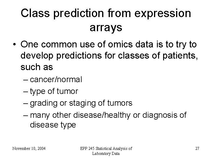
Class prediction from expression arrays • One common use of omics data is to try to develop predictions for classes of patients, such as – cancer/normal – type of tumor – grading or staging of tumors – many other disease/healthy or diagnosis of disease type November 10, 2004 EPP 245 Statistical Analysis of Laboratory Data 27

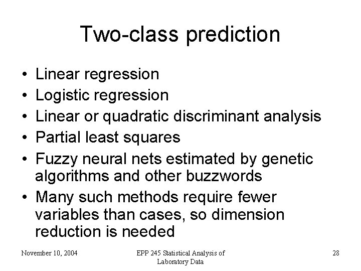
Two-class prediction • • • Linear regression Logistic regression Linear or quadratic discriminant analysis Partial least squares Fuzzy neural nets estimated by genetic algorithms and other buzzwords • Many such methods require fewer variables than cases, so dimension reduction is needed November 10, 2004 EPP 245 Statistical Analysis of Laboratory Data 28

Dimension Reduction • Suppose we have 20, 000 variables and wish to predict whether a patient has ovarian cancer or not and suppose we have 50 cases and 50 controls • We can only use a number of predictors much smaller than 50 • How do we do this? November 10, 2004 EPP 245 Statistical Analysis of Laboratory Data 29

• Two distinct ways are selection of genes and selection of “supergenes” as linear combinations • We can choose the genes with the most significant t-tests or other individual gene criteria • We can use forward stepwise logistic regression, which adds the most significant gene, then the most significant addition, and so on, or other ways of picking the best subset of genes November 10, 2004 EPP 245 Statistical Analysis of Laboratory Data 30

Supergenes are linear combinations of genes. If g 1, g 2, g 3, …, gp are the expression measurements for the p genes in an array, and a 1, a 2, a 3, …, ap are a set of coefficients then g 1 a 1+ g 2 a 2+ g 3 a 3+ …+ gp ap is a supergene. Methods for construction of supergenes include PCA and PLS November 10, 2004 EPP 245 Statistical Analysis of Laboratory Data 31

Choosing Subsets of Supergenes • Suppose we have 50 cases and 50 controls and an array of 20, 000 gene expression values for each of the 100 observations • In general, any arbitrary set of 100 genes will be able to predict perfectly in the data if a logistic regression is fit to the 100 genes • Most of these will predict poorly in future samples November 10, 2004 EPP 245 Statistical Analysis of Laboratory Data 32

• This is a mathematical fact • A statistical fact is that even if there is no association at all between any gene and the disease, often a few genes will produce apparently excellent results, that will not generalize at all • We must somehow account for this, and cross validation is the usual way November 10, 2004 EPP 245 Statistical Analysis of Laboratory Data 33

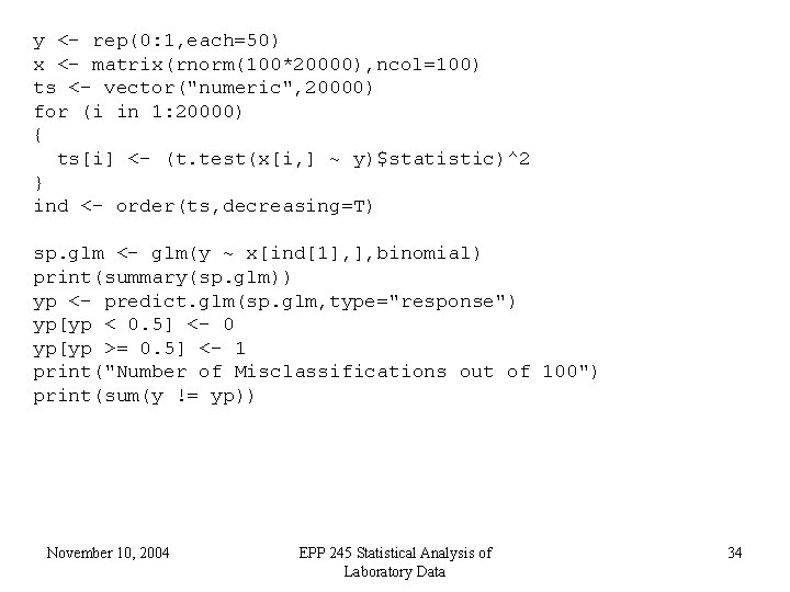
y <- rep(0: 1, each=50) x <- matrix(rnorm(100*20000), ncol=100) ts <- vector("numeric", 20000) for (i in 1: 20000) { ts[i] <- (t. test(x[i, ] ~ y)$statistic)^2 } ind <- order(ts, decreasing=T) sp. glm <- glm(y ~ x[ind[1], ], binomial) print(summary(sp. glm)) yp <- predict. glm(sp. glm, type="response") yp[yp < 0. 5] <- 0 yp[yp >= 0. 5] <- 1 print("Number of Misclassifications out of 100") print(sum(y != yp)) November 10, 2004 EPP 245 Statistical Analysis of Laboratory Data 34

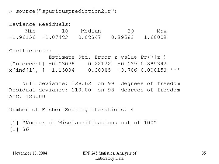
> source("spuriousprediction 2. r") Deviance Residuals: Min 1 Q -1. 96156 -1. 07483 Median 0. 08347 3 Q 0. 99583 Max 1. 68009 Coefficients: Estimate Std. Error z value Pr(>|z|) (Intercept) -0. 03078 0. 22122 -0. 139 0. 889342 x[ind[1], ] -1. 15034 0. 30385 -3. 786 0. 000153 *** Null deviance: 138. 63 Residual deviance: 119. 00 AIC: 123. 00 on 99 on 98 degrees of freedom Number of Fisher Scoring iterations: 4 [1] "Number of Misclassifications out of 100" [1] 36 November 10, 2004 EPP 245 Statistical Analysis of Laboratory Data 35

[1] "Number of variables/Misclassifications out of 100" [1] 1 36 [1] "Number of variables/Misclassifications out of 100" [1] 2 32 [1] "Number of variables/Misclassifications out of 100" [1] 3 27 [1] "Number of variables/Misclassifications out of 100" [1] 4 19 [1] "Number of variables/Misclassifications out of 100" [1] 5 17 [1] "Number of variables/Misclassifications out of 100" [1] 6 21 [1] "Number of variables/Misclassifications out of 100" [1] 7 16 [1] "Number of variables/Misclassifications out of 100" [1] 20 0 Warning messages: 1: Algorithm did not converge in: glm. fit(x = X, y = Y, weights = weights, start = start, etastart = etastart, 2: fitted probabilities numerically 0 or 1 occurred in: glm. fit(x = X, y = Y, weights = weights, start = start, etastart = etastart, November 10, 2004 EPP 245 Statistical Analysis of Laboratory Data 36

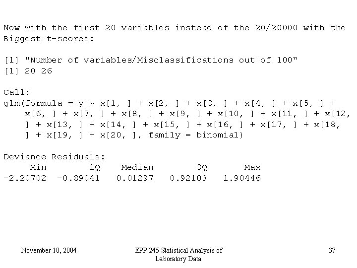
Now with the first 20 variables instead of the 20/20000 with the Biggest t-scores: [1] "Number of variables/Misclassifications out of 100" [1] 20 26 Call: glm(formula = y ~ x[6, ] + x[7, ] + x[13, ] + x[19, ] + x[1, ] + x[2, ] + x[8, ] + x[9, x[14, ] + x[15, ] x[20, ], family = Deviance Residuals: Min 1 Q -2. 20702 -0. 89041 November 10, 2004 Median 0. 01297 x[3, ] + x[4, ] + x[5, ] + x[10, ] + x[11, ] + x[12, + x[16, ] + x[17, ] + x[18, binomial) 3 Q 0. 92103 EPP 245 Statistical Analysis of Laboratory Data Max 1. 90446 37

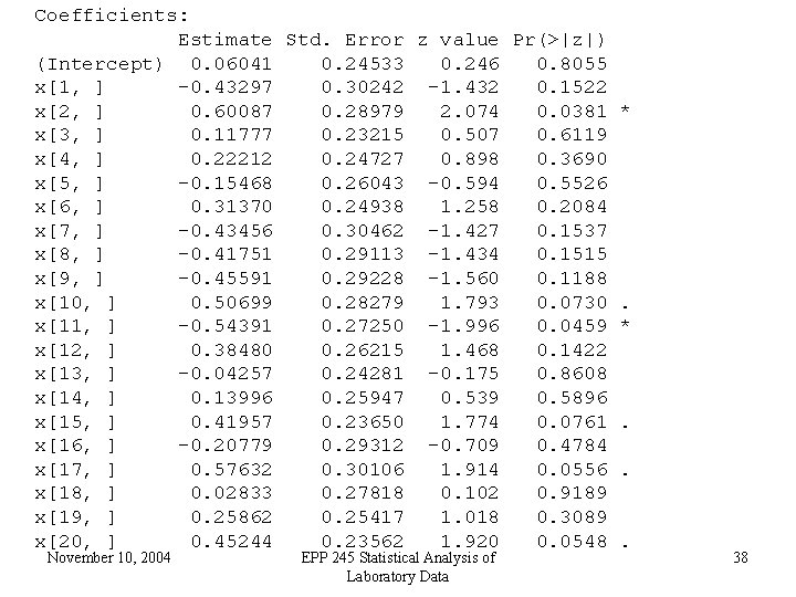
Coefficients: Estimate Std. Error z value Pr(>|z|) (Intercept) 0. 06041 0. 24533 0. 246 0. 8055 x[1, ] -0. 43297 0. 30242 -1. 432 0. 1522 x[2, ] 0. 60087 0. 28979 2. 074 0. 0381 * x[3, ] 0. 11777 0. 23215 0. 507 0. 6119 x[4, ] 0. 22212 0. 24727 0. 898 0. 3690 x[5, ] -0. 15468 0. 26043 -0. 594 0. 5526 x[6, ] 0. 31370 0. 24938 1. 258 0. 2084 x[7, ] -0. 43456 0. 30462 -1. 427 0. 1537 x[8, ] -0. 41751 0. 29113 -1. 434 0. 1515 x[9, ] -0. 45591 0. 29228 -1. 560 0. 1188 x[10, ] 0. 50699 0. 28279 1. 793 0. 0730. x[11, ] -0. 54391 0. 27250 -1. 996 0. 0459 * x[12, ] 0. 38480 0. 26215 1. 468 0. 1422 x[13, ] -0. 04257 0. 24281 -0. 175 0. 8608 x[14, ] 0. 13996 0. 25947 0. 539 0. 5896 x[15, ] 0. 41957 0. 23650 1. 774 0. 0761. x[16, ] -0. 20779 0. 29312 -0. 709 0. 4784 x[17, ] 0. 57632 0. 30106 1. 914 0. 0556. x[18, ] 0. 02833 0. 27818 0. 102 0. 9189 x[19, ] 0. 25862 0. 25417 1. 018 0. 3089 x[20, ] 0. 45244 0. 23562 1. 920 0. 0548. November 10, 2004 EPP 245 Statistical Analysis of Laboratory Data 38

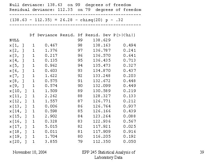
Null deviance: 138. 63 on 99 degrees of freedom Residual deviance: 112. 35 on 79 degrees of freedom --------------------------(138. 63 – 112. 35) = 26. 28 ~ chisq(20) p ~. 32 --------------------------NULL x[1, ] x[2, ] x[3, ] x[4, ] x[5, ] x[6, ] x[7, ] x[8, ] x[9, ] x[10, ] x[11, ] x[12, ] x[13, ] x[14, ] x[15, ] x[16, ] x[17, ] x[18, ] x[19, ] x[20, ] Df Deviance Resid. Df Resid. Dev P(>|Chi|) 99 138. 629 1 0. 467 98 138. 163 0. 494 1 1. 376 97 136. 787 0. 241 1 0. 217 96 136. 570 0. 641 1 0. 135 95 136. 435 0. 713 1 0. 962 94 135. 473 0. 327 1 0. 603 93 134. 870 0. 437 1 1. 622 92 133. 248 0. 203 1 0. 575 91 132. 672 0. 448 1 0. 574 90 132. 099 0. 449 1 1. 509 89 130. 589 0. 219 1 2. 262 88 128. 327 0. 133 1 1. 557 87 126. 771 0. 212 1 0. 006 86 126. 764 0. 937 1 0. 598 85 126. 166 0. 439 1 2. 902 84 123. 264 0. 088 1 0. 328 83 122. 936 0. 567 1 5. 015 82 117. 921 0. 025 1 0. 011 81 117. 909 0. 916 1 1. 704 80 116. 205 0. 192 1 3. 855 79 112. 350 0. 050 November 10, 2004 EPP 245 Statistical Analysis of Laboratory Data 39

Consequences of many variables • If there is no effect of any variable on the classification, it is still the case that the number of cases correctly classified increases in the sample that was used to derive the classifier as the number of variables increases • But the statistical significance is usually not there November 10, 2004 EPP 245 Statistical Analysis of Laboratory Data 40

• If the variables used are selected from many, the apparent statistical significance and the apparent success in classification is greatly inflated, causing end-stage delusionary behavior in the investigator • This problem can be improved using cross validation or other resampling methods November 10, 2004 EPP 245 Statistical Analysis of Laboratory Data 41

Overfitting • When we fit a statistical model to data, we adjust the parameters so that the fit is as good as possible and the errors are as small as possible • Once we have done so, the model may fit well, but we don’t have an unbiased estimate of how well it fits if we use the same data to assess as to fit November 10, 2004 EPP 245 Statistical Analysis of Laboratory Data 42

Training and Test Data • One way to approach this problem is to fit the model on one dataset (say half the data) and assess the fit on another • This avoids bias but is inefficient, since we can only use perhaps half the data for fitting • We can get more by doing this twice in which each half serves as the training set once and the test set once • This is two-fold cross validation November 10, 2004 EPP 245 Statistical Analysis of Laboratory Data 43

• It may be more efficient to use 5 - 10 -, or 20 -fold cross validation depending on the size of the data set • Leave-out-one cross validation is also popular, especially with small data sets • With 10 -fold CV, one can divide the set into 10 parts, pick random subsets of size 1/10, or repeatedly divide the data November 10, 2004 EPP 245 Statistical Analysis of Laboratory Data 44

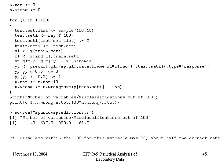
n. tot <- 0 n. wrong <- 0 for (i in 1: 100) { test. set. list <- sample(100, 10) test. seti <- rep(F, 100) test. seti[test. set. list] <- T train. seti <- !test. seti y 1 <- y[train. seti] x 1 <- x[ind[1], train. seti] sp. glm <- glm( y 1 ~ x 1, binomial) yp <- predict. glm(sp. glm, data. frame(x 1=x[ind[1], test. seti]), type="response") yp[yp < 0. 5] <- 0 yp[yp >= 0. 5] <- 1 n. tot <- n. tot+10 n. wrong <- n. wrong+sum(y[test. seti] == yp) } print("Number of variables/Misclassifications out of 100") print(c(1, n. wrong, n. tot, 100*n. wrong/n. tot)) > source("spuriousprediction 3. r") [1] "Number of variables/Misclassifications out of 100" [1] 1. 0 637. 0 1000. 0 63. 7 Cf. missclass within the 100 for this variable was 36, about half the correct rate November 10, 2004 EPP 245 Statistical Analysis of Laboratory Data 45

Stepwise Logistic Regression • Another way to select variables is stepwise • This can be better than individual variable selection, which may choose many highly correlated predictors that are redundent • A generic function step() can be used for many kinds of predictor functions in R November 10, 2004 EPP 245 Statistical Analysis of Laboratory Data 46

Using step() • step(glm. model) is sufficient • It uses steps either backward (using drop 1) or forward (using add 1) until a model is reached that cannot be improved • Criterion is AIC = Akaiki Information Criterion, which tries to account for the effect of extra variables, more so than MSE or R 2 November 10, 2004 EPP 245 Statistical Analysis of Laboratory Data 47

• You may also specify a scope in the form of a list(lower=model 1, upper =model 2) • For expression arrays, with thousands of variables one should start with y ~ 1 and use scope =list(lower=y~1, upper=**) November 10, 2004 EPP 245 Statistical Analysis of Laboratory Data 48

for (i in 1: 100) { assign(paste("x", i, sep=""), x[ind[i], ]) } fchar <- "y~x 1" for (i in 2: 100) { fchar <- paste(fchar, "+x", i, sep="") } form <- as. formula(fchar) step(glm(y ~ 1), list(lower=(y~1), upper=form)) November 10, 2004 EPP 245 Statistical Analysis of Laboratory Data 49

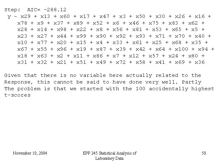
Step: AIC= -288. 12 y ~ x 29 + x 13 + x 60 + x 17 + x 47 + x 3 + x 50 + x 30 + x 26 + x 16 + x 78 + x 9 + x 37 + x 89 + x 52 + x 6 + x 46 + x 75 + x 83 + x 62 + x 28 + x 14 + x 98 + x 22 + x 8 + x 56 + x 81 + x 53 + x 65 + x 23 + x 27 + x 44 + x 99 + x 90 + x 92 + x 93 + x 71 + x 70 + x 40 + x 10 + x 77 + x 20 + x 15 + x 4 + x 33 + x 61 + x 25 + x 68 + x 35 + x 67 + x 55 + x 96 + x 19 + x 87 + x 39 + x 42 + x 64 + x 100 + x 94 + x 18 + x 63 + x 2 + x 11 + x 86 + x 7 + x 12 + x 57 + x 24 + x 80 + x 31 + x 32 + x 21 + x 51 + x 49 + x 72 + x 58 + x 41 + x 69 + x 36 Given that there is no variable here actually related to the Response, this cannot be said to have done very well. Partly The problem is that we started with the 100 accidentally highest t-scores November 10, 2004 EPP 245 Statistical Analysis of Laboratory Data 50

Exercises • Do problems 11. 1 -11. 3 in Dalgaard. November 10, 2004 EPP 245 Statistical Analysis of Laboratory Data 51